MMM fundamentals
Adstock and saturation explained in plain terms
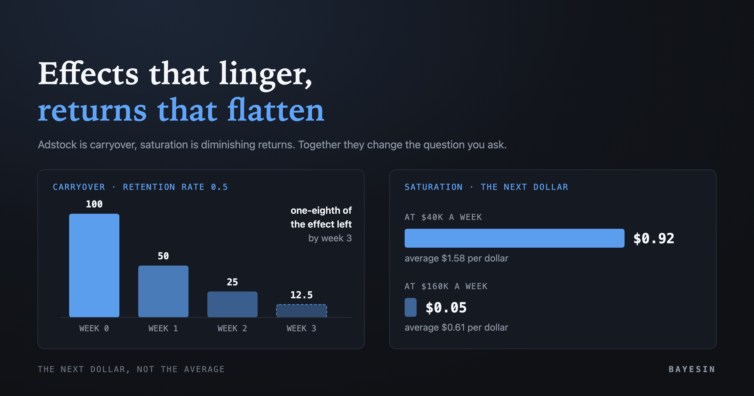
Adstock and saturation explained in plain terms: a 0.5 retention rate leaves one-eighth of an ad's effect by week 3, and the next dollar can return $0.05.
Brandon Cade · Sep 24, 2026 · 9 min read
Key Takeaways
- Adstock is carryover. Part of this week's spend keeps working later, and the model estimates how much and for how long.
- Saturation is diminishing returns. Each extra dollar in a channel usually works a little less than the one before.
- Together they turn one question, "what did this channel return?", into two: what did it return so far, and what will the next dollar return?
- Both curves are estimated, not observed. Read them with their credible intervals, and stay near the spend range the data actually covers.
Most of what a media mix model tells you comes down to two ideas. A dollar continues to work after you spend it, and each additional dollar works somewhat less effectively than the one before. The first idea is called adstock and the second is called saturation. This guide gives adstock and saturation explained through one small example, and then shows how to test whether a model's curves deserve your trust.
What is adstock, and why does a model need it?
Adstock is the proportion of one week's advertising effect that carries into later weeks. Someone who sees an ad on Tuesday may not purchase until next week. A model that compares only this week's spend with this week's revenue misses that delay. It can then under-credit a channel or assign the credit to whatever happened to run when the sale occurred.
In 2017, Google researchers Yuxue Jin and colleagues noted that advertising usually has lag effects. A model therefore needs a way to let past spend influence present revenue, which their paper calls the carryover effect. The paper is Google Research's "Bayesian Methods for Media Mix Modeling with Carryover and Shape Effects."
The simplest form is geometric adstock, in which each week keeps a fixed share of the previous week's effect, called the retention rate. The PyMC-Marketing guide to adstock transformations writes the rule as this week's spend plus the retention rate times last week's adstocked value. A retention rate of 0.5 means half the effect survives each week, and a rate of 0.8 means four-fifths survives.
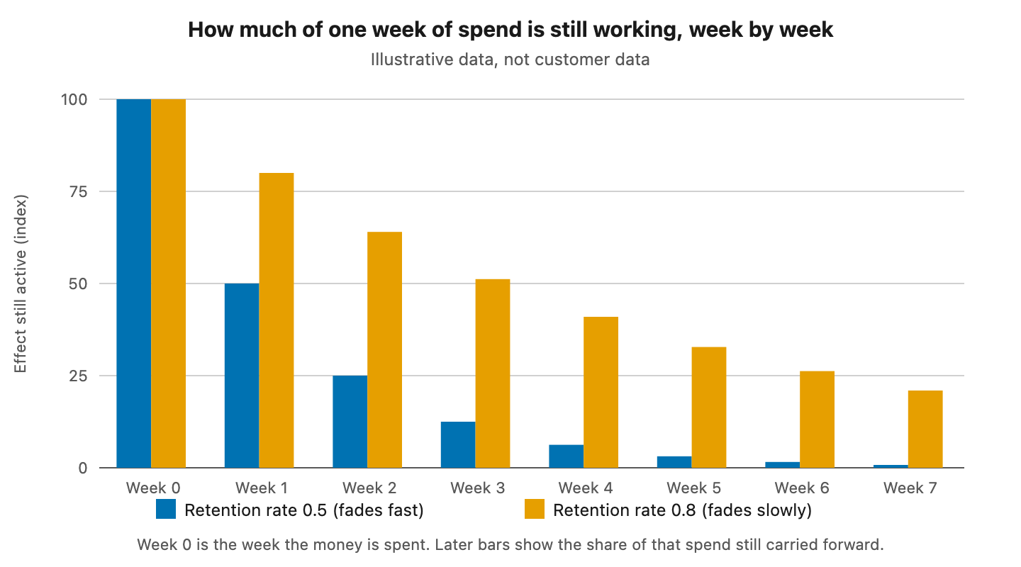
Figure 1. Carryover of a single week of spend. Illustrative numbers, not real customer data.
The chart shows why the choice matters. With a retention rate of 0.5, the effect in week 3 is one-eighth of the original, but with 0.8 it is still about half. Two channels with the same weekly spend can therefore deserve very different credit windows.
Saturation is diminishing returns, and the curve bends
Saturation means that each additional dollar in a channel usually drives less revenue than the dollar before it. The first dollars reach the people most ready to act, and later dollars reach people who are harder to persuade. Plotted, revenue rises steeply at first, then bends and flattens toward a ceiling.
Google's Meridian documentation says that as spending on a channel rises, you eventually see diminishing marginal returns, which it calls saturation. As of September 2026, Meridian models this with a Hill function that has two parameters. One sets the half-saturation point, the spend at which the channel reaches half of its ceiling. The other sets whether the curve is concave or S-shaped.
PyMC-Marketing's saturation tutorial describes the same effect with a logistic curve. It has one parameter for the ceiling, the most a channel can contribute, and one for how fast the curve approaches that ceiling. The tools differ in functional form, but most media mix models include some version of a curve that bends.
Adstock and saturation explained: how the two ideas work together
Adstock changes when spend counts, whereas saturation changes how much each unit of spend counts. A model applies both transformations to a channel's spend before it estimates the channel's contribution. The resulting curve describes revenue as a function of effective spend, not of the raw dollars on that week's invoice.
You can think of them as two dials per channel. One dial sets how long the effect persists, and the other sets how quickly the channel exhausts its most responsive customers.
The pair also changes budget decisions. Average return answers what a channel did over a period. Marginal return is the slope of the curve at today's spend, once carryover is included, and it answers what the next dollar will do. Reallocation should follow that second number. I go deeper on the split in marginal ROAS vs average ROAS.
Open-source tools offer a small menu of curve shapes
Open-source tools offer a small menu of shapes for both dials. Geometric adstock is the common default, and the alternatives add a delay before the peak or a more flexible tail. For saturation, the Hill and logistic curves dominate. The table summarizes what each project's public documentation describes.
- Meta Robyn — Carryover forms: Geometric; Weibull (two variants); Saturation forms: Hill, with shape and inflection parameters
- Google Meridian — Carryover forms: Weighted average of current and earlier weeks; Saturation forms: Hill, with half-saturation and slope
- PyMC-Marketing — Carryover forms: Geometric; delayed; Weibull (two variants); Saturation forms: Logistic, with ceiling and rate parameters
Sources: Robyn "Key Features"; Meridian "Media saturation and lagging"; PyMC-Marketing adstock guide and saturation tutorial. The table compares what each page describes and does not rank the tools.
Robyn's documentation notes that the Weibull options allow a lagged peak, which suits media where awareness builds before it converts. The PyMC-Marketing guide makes the same point about delayed adstock for traditional media. A geometric shape peaks in the week of spend, so it suits channels where the response is immediate.
One channel at two spend levels: the next dollar falls from $0.92 to $0.05
The example below uses synthetic numbers, so they are illustrative and not real customer data. Suppose a channel's weekly revenue follows a saturation curve. Driven revenue equals 100 times one minus the exponential of negative spend divided by 40, with both figures in thousands of dollars.
At $40 thousand a week, the curve gives about $63 thousand of driven revenue. Average return is about $1.58 per dollar, and the slope is steep: the next dollar returns about $0.92. At $160 thousand a week, the curve gives about $98 thousand. Average return has fallen to about $0.61, and the next dollar now returns about $0.05.
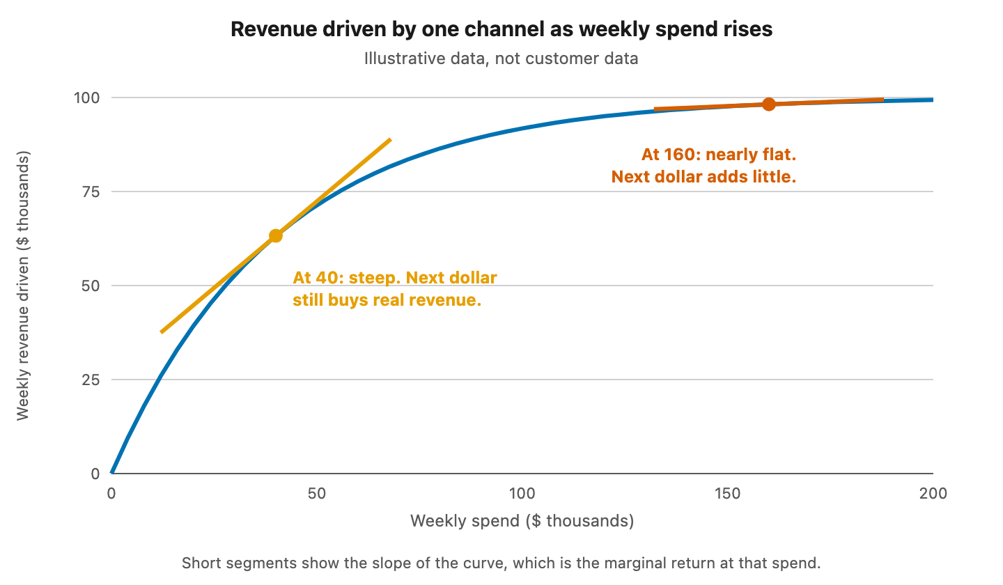
Figure 2. A saturation curve with the slope marked at two spend levels. Illustrative numbers, not real customer data.
Quadrupling spend added only about $35 thousand of driven revenue. Now add carryover. With a retention rate of 0.5, one week of $100 spend leaves an effect of 100, 50, 25 and 12.5 over the first four weeks. The total over eight weeks is about 199. A model without adstock would have booked only the first week's 100 to that channel.
The lesson is not that the channel at $160 thousand is broken. Its next dollar is worth far less than its average dollar, and only a response curve makes that difference visible.
What can go wrong when you read these curves?
Three limits matter most. First, the curves are estimated from the range of spend the data contains. Second, priors carry more weight when data is thin, and third, channels that move together are hard to separate. Each limit has a verification you can perform before you act on a curve.
Meridian's documentation is explicit about the first limit. It states that its Hill parameter estimates rest on the observed range of media data. Results based on extrapolation should be read with appropriate caution. If a channel has never been near $200 thousand a week, the right side of its curve is a projection and not a measurement.
The second limit comes from the 2017 Jin paper, which reports that priors influence results significantly with smaller samples and can cause bias. I explain what that means in priors in a Bayesian marketing mix model. How it differs under a regression fit is in Bayesian vs frequentist MMM.
The third limit is older. Chan and Perry's 2017 paper lists correlated input variables among the challenges of media mix modeling, and the pillar guide gives the source. When two channels rise and fall together, the model may apportion their credit in ways the data cannot settle.
How can you test whether the curves are believable?
Ask for three pieces of evidence: the credible interval on each curve parameter, the spend range the data covers, and an outside check. A wide interval says the data cannot pin the curve down. A curve read far outside observed spend is a projection. An experiment is the outside check, because it measures the effect directly.
Four questions cover the ground when you look at any set of curves:
- What is the credible interval on the carryover and the saturation parameters, and not only the central estimate?
- What weekly spend range did the model actually see for this channel?
- Do the curves agree with any holdout or lift test you have run?
- Does the ranking of channels by marginal return change if you move the carryover assumption?
The third question has support in the literature. In 2024, Google researchers Yingxiang Zhang and colleagues proposed setting priors so that experiment results can inform an MMM directly. Their paper is "Media Mix Model Calibration With Bayesian Priors." In simulations, they report that the approach substantially decreases bias and uncertainty in posterior return estimates. Robyn's documentation likewise supports calibrating a model with sales and geo experiments.
For the same idea in everyday language, read Diminishing returns: why the tenth dollar works less than the first.
Frequently asked questions
Is adstock the same as attribution windows?
No. An attribution window is a rule, chosen by a person, that credits a conversion to ads seen within a fixed number of days. Adstock is an estimated decay curve fitted to weekly spend and revenue. The retention rate comes from the data, with a credible interval that shows how sure the model is.
Does saturation mean I should stop spending in a channel?
Not by itself. Saturation means the next dollar returns less than the average dollar. Whether that next dollar is still worth spending depends on what it returns compared with your other options and your margin. Compare marginal returns across channels, with their credible intervals, before moving any budget.
How many weeks of data do these curves need?
More than a few months. Carryover and saturation are estimated per channel, so each channel needs both enough weeks and enough movement in its spend. Meridian's documentation adds that estimates rest on the observed range of spend. The pillar guide covers data requirements in more detail.
Can a model choose the wrong curve shape?
Yes. If the data cannot distinguish a geometric decay from a delayed one, two shapes can fit about equally well and imply different budget advice. Comparing fits, checking against experiments, and reading the interval on the peak week are the practical defenses against choosing the wrong one.
Sources
- Google Research, Jin, Wang, Sun, Chan and Koehler, "Bayesian Methods for Media Mix Modeling with Carryover and Shape Effects"
- Google Research, Chan and Perry, "Challenges and Opportunities in Media Mix Modeling"
- Google Research, Zhang et al., "Media Mix Model Calibration With Bayesian Priors"
- Google for Developers, "Media saturation and lagging," Meridian documentation
- Meta, "Key Features," Robyn documentation
- PyMC-Marketing, "Guide to Adstock Transformations"
- PyMC-Marketing, "Understanding Media Saturation in Marketing Mix Models"
See it on your own rows.
Bayesin is pre-launch. Join the waitlist and we will reach out as access opens.
Get new posts by email.
New posts only. See privacy for what we keep.