Bayesian vs frequentist MMM: what changes on the page

Key Takeaways

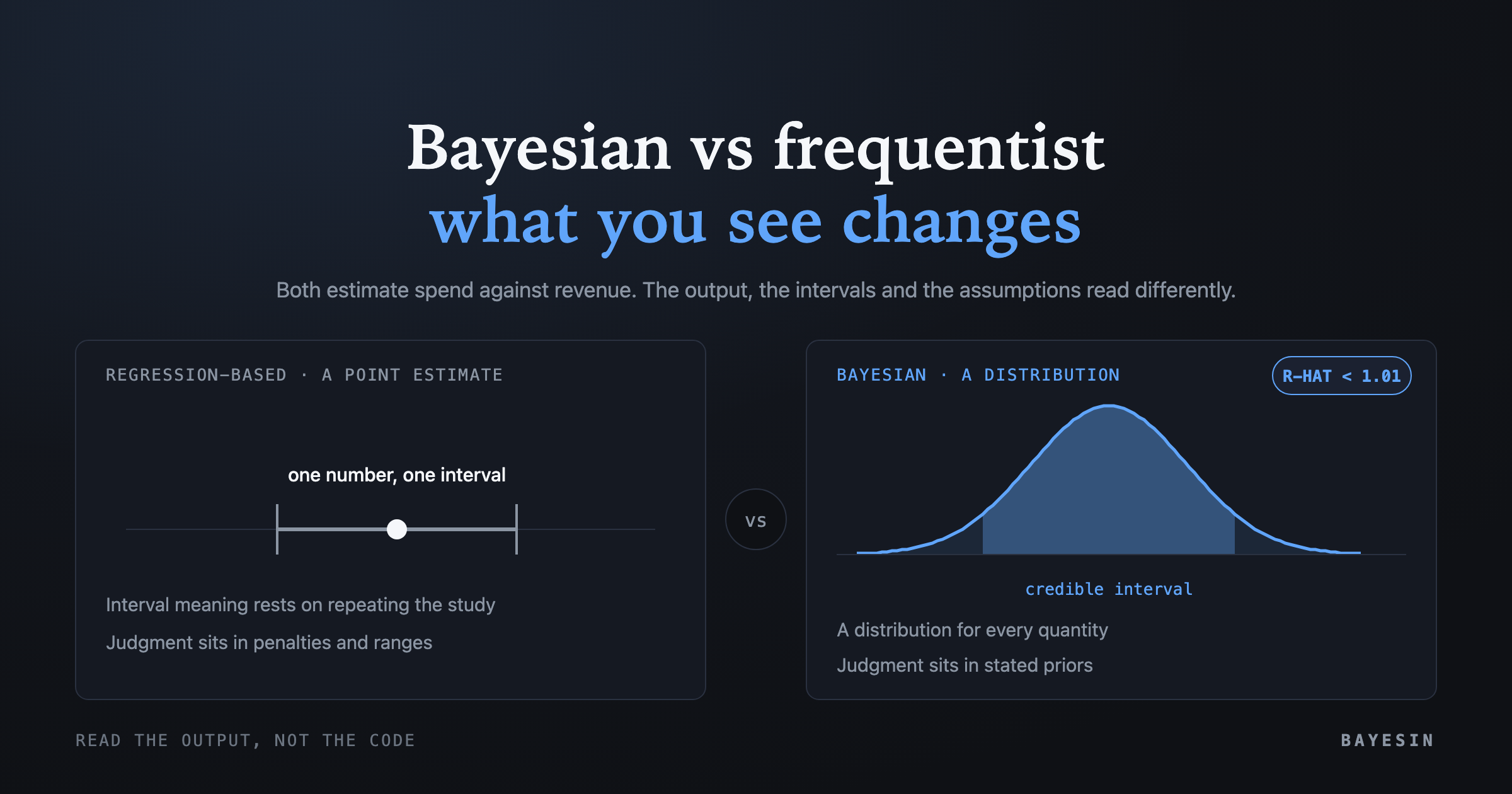
• • The main difference you see is the output. A Bayesian MMM returns a distribution for each quantity, so a credible interval reads as a direct probability statement.
  • A Bayesian model states its assumptions up front as priors. Other approaches put comparable judgment in hyperparameter ranges, penalties and model selection.
  • With thin data, priors carry more weight. That is a reason to read them, not a reason to avoid the method.
  • Neither approach removes confounding. Both need good controls, enough variation in spend, and an outside check.

This is a comparison for the person reading the output, not the person writing the code. Bayesian vs frequentist MMM is a question about what you get back, how uncertainty is expressed, and where the modeler's assumptions sit. Both families estimate how spend relates to revenue, and both are used seriously in practice, so I compare them on those terms.

What does "frequentist" mean in this comparison?

In frequentist inference, a parameter is a fixed unknown. An estimate comes with a confidence interval whose meaning rests on repeating the study many times. Jonathan Bartlett describes this contrast with credible intervals in his post on The Stats Geek.

Meta's Robyn documentation never calls the tool frequentist. It describes ridge regression with candidate models chosen by the analyst. I group such penalized-regression tools under the loose label because they return point estimates with no posterior distribution. I say "regression-based" whenever the distinction matters. Individual products vary, so read the label as a way to organize the comparison and not as a classification of any vendor.

Bayesian vs frequentist MMM: what a Bayesian fit adds

A Bayesian model starts with a prior, a stated belief about each parameter before seeing your data. It then updates that belief with your weekly rows and returns a posterior distribution. You get a range of plausible values with a probability attached, instead of one best-fit number.

In 2017, Google researchers Yuxue Jin and colleagues proposed this setup for media mix modeling. Their paper is "Bayesian Methods for Media Mix Modeling with Carryover and Shape Effects," and its model uses prior information from historical or related campaigns. The posterior then supports metrics such as return on ad spend and marginal return, each with a distribution behind it.

As of September 2026, Google's Meridian documentation describes the same idea. It says a Bayesian regression model combines prior knowledge with signals learned from data, and that it uses MCMC sampling to estimate all coefficients together. MCMC is a way of drawing many samples from the posterior.

How do the two kinds of intervals read differently?

A frequentist confidence interval describes a procedure. A Bayesian credible interval describes the parameter itself, given the data and the prior. It supports a direct statement such as "there is an 80% probability that this value lies in this range." That is the practical reason I use the term credible interval throughout this cluster.

Bartlett's post, first published in 2020 and updated in 2024, sets out the difference. For a confidence interval, the claim is about repetition. If the assumptions hold and you repeated the study many times, a stated share of the intervals would contain the true value. For any single interval, you cannot say whether it does.

For a credible interval, you can state the probability that the value lies inside it, conditional on the model and the prior. Bartlett is careful to note that this probability carries its own interpretive caveats. The practical gain is simpler wording, not a guarantee.

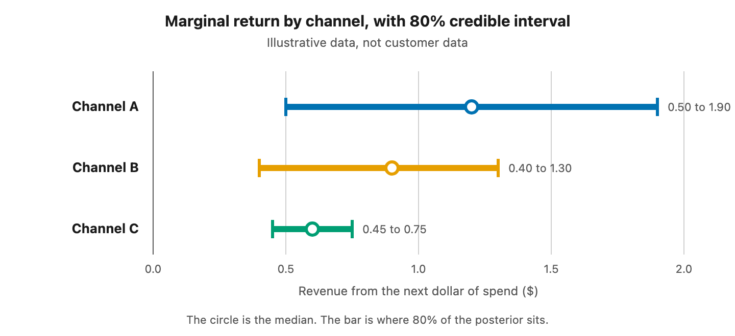
Figure 1. A credible interval on marginal return by channel.

The figure shows why the interval matters more than the ranking. Channel A has the highest median but the widest interval, and it overlaps Channel B. A report that shows only medians would present a clean ranking that the data does not support.

Each approach puts the modeler's judgment in a different place

Every MMM embeds judgment. A Bayesian model puts it in priors that can be listed and challenged. A regression-based tool such as Robyn puts comparable judgment into hyperparameter bounds, a ridge penalty, and the analyst's choice among candidate models. The difference is visibility, not the presence of judgment.

Robyn's analyst guide describes ridge regression as built in to handle multicollinearity, using a regularization technique that reduces variance at the cost of some bias. Robyn generates a series of Pareto-optimal candidate models, and users pick the final one using business judgment, experiments and statistical parameters.

The Bayesian route makes those choices explicit. Google's Meridian documentation lists priors for media effects, adstock decay, saturation parameters and residual variance. It also lets you set priors on return on investment or marginal return, so that domain knowledge enters in a unit a marketer can check.

The Stan project's prior guidance suggests a useful bar. In a version edited in April 2025, it advises that informative priors be made explicit, with a sentence written about each parameter. I take that as the standard for any MMM: if a model has assumptions, the reader should be able to find them. I cover this in priors in a Bayesian marketing mix model.

Thin data is where the two approaches diverge

Thin data is where the two approaches diverge most in practice. A Bayesian model leans more on its priors when the data says little and more on the data when it says a lot. That is a feature when the priors are sensible and a hazard when they are careless.

The Jin paper reports this trade-off in its abstract. The model performs well with large datasets, but priors significantly influence results with smaller samples and can cause bias. The paper also flags the variance of recommended budget allocations as a challenge, which is why intervals matter for decisions.

Google's 2017 geo-level paper, by Yunting Sun and colleagues, describes national-level MMMs as often suffering from small sample size and insufficient variation in media spend. Its hierarchical model produced tighter credible intervals by using regional data. Regression-based tools face the same scarcity, and ridge shrinkage plays a role similar to a prior.

Side by side: what the reader sees

The table compares what a reader typically sees from a Bayesian MMM and from a regression-based tool such as Robyn. It compares published documentation and does not rank the approaches. Individual products vary, and every Robyn row draws on its own guide.

• What comes back? — Bayesian MMM: A posterior distribution for each parameter and metric; Regression-based MMM (Robyn as example): A set of candidate models to choose from
• How is uncertainty shown? — Bayesian MMM: Credible intervals on channel figures; Regression-based MMM (Robyn as example): Depends on the tool; candidates differ in fit and decomposition
• Where do assumptions live? — Bayesian MMM: Priors, listed per parameter; Regression-based MMM (Robyn as example): Hyperparameter bounds, ridge penalty, model selection
• How do experiments enter? — Bayesian MMM: Through priors on return or marginal return; Regression-based MMM (Robyn as example): Through calibration on sales or geo experiments
• How does thin data behave? — Bayesian MMM: Priors carry more weight; intervals widen; Regression-based MMM (Robyn as example): Regularization shrinks minor coefficients
• How is a run checked? — Bayesian MMM: Sampler diagnostics such as R-hat; Regression-based MMM (Robyn as example): Fit error and decomposition measures

Sources: Meridian documentation; Robyn "Key Features" and analyst guide; Jin et al. (2017).

Both columns can use experiments. In 2024, Yingxiang Zhang and colleagues at Google showed how to fold experiment results into a Bayesian MMM by putting the prior on return itself. Robyn's documentation describes calibrating with sales and geo experiments. Either way, an experiment is the strongest outside check available.

The hard problems are the same in both

The hard problems are the same. Chan and Perry laid out in 2017 why any media mix model struggles to answer an advertiser's questions consistently. Limited data, correlated input variables and selection bias are among the reasons. The pillar guide gives that source. Switching estimators does not remove these obstacles.

Meridian's documentation makes a related point about controls. It says control variables estimate baseline outcome and that confounders, the variables affecting both spend and the outcome, should be included to debias causal estimates. It also warns that control coefficients cannot be read as causal effects. I treat this at length in MMM baseline, seasonality and promotions.

Carryover and saturation also work the same way in both families, as I describe in adstock and saturation explained. The choice of estimator changes how you read the uncertainty, not what the curves mean.

How can you evaluate any MMM's output?

Ask five questions of any MMM, Bayesian or not. What assumptions does it make, and where are they written? Does each channel figure carry an interval? Was the fit checked, and how? Did any outside experiment inform it? What would make the model refuse to answer?

For Bayesian fits, the check has a standard form. The Stan reference manual notes that Vehtari and colleagues suggest a general R-hat threshold of 1.01 for judging whether chains have converged. Their 2021 paper in Bayesian Analysis showed that the traditional R-hat can miss convergence problems when chains have heavy tails or differing variances.

The answer to the last question matters most for any approach. A modeling process that can never say "the data cannot support this" will always give you a number. The pillar guide explains why I think a model that can refuse is easier to defend.

Frequently asked questions

Is one approach more accurate than the other?

Neither wins in general. Accuracy depends on data quality, spend variation, controls and how well the model form matches reality. The Bayesian approach gives you intervals and stated priors, and regression-based tools can be equally sound. Judge a model by its out-of-sample checks and any experiments, not by its label.

Do Bayesian models need a lot more data?

Not necessarily more, but they use it differently. With little data the prior dominates, so results lean on assumptions you can see, and with more data the data dominates. The 2017 Jin paper found that priors matter most in small samples. Any MMM with thin data will have wide uncertainty.

Can a Bayesian model be biased by its priors?

Yes, especially on small samples, as Jin and colleagues found. The defenses are to use weakly informative priors, document them, compare results under different priors, and calibrate against experiments wherever you can run them. A stated prior can be tested, whereas a hidden assumption cannot be inspected at all.

Why not just report one best number?

A single number hides how sure the model is. Two channels with medians of 1.2 and 0.9 may be indistinguishable once their intervals are drawn. Intervals let you see when a reallocation has support and when it is closer to a coin flip.

Sources

• Google Research, Jin, Wang, Sun, Chan and Koehler, "Bayesian Methods for Media Mix Modeling with Carryover and Shape Effects"
• Google Research, Sun, Wang, Jin, Chan and Koehler, "Geo-level Bayesian Hierarchical Media Mix Modeling"
• Google Research, Chan and Perry, "Challenges and Opportunities in Media Mix Modeling"
• Google Research, Zhang et al., "Media Mix Model Calibration With Bayesian Priors"
• Google for Developers, "Bayesian Inference in Meridian," Meridian documentation
• Google for Developers, "Control variables," Meridian documentation
• Google for Developers, "Choose and configure treatment prior types," Meridian documentation
• Meta, "Analyst's guide to MMM," Robyn documentation
• Meta, "Key Features," Robyn documentation
• Stan Development Team, "Prior Choice Recommendations"
• Stan Development Team, "Stan Reference Manual: Posterior Analysis"
• Bartlett, "Interpretation of frequentist confidence intervals and Bayesian credible intervals," The Stats Geek
• Vehtari, Gelman, Simpson, Carpenter and Bürkner, "Rank-normalization, folding, and localization: An improved R-hat for assessing convergence of MCMC," Bayesian Analysis