MMM fundamentals
Media mix modeling explained for the budget owner
Media mix modeling explained for the person defending a budget: the data, the method, the outputs, and ten questions plus a 1.01 R-hat check for trust.
Brandon Cade · Sep 27, 2026 · 15 min read
Key Takeaways
- A media mix model (MMM) uses weekly spend and revenue to estimate what each channel drives, and what the next dollar in each channel is likely to return.
- Four ideas do most of the work: carryover, diminishing returns, a baseline of demand that would arrive anyway, and seasonality.
- The most useful outputs are marginal return, baseline share and channel contribution, each reported with a credible interval instead of a single number.
- A model can be wrong without looking wrong, so ask how it was checked, what it assumed, and whether it is allowed to refuse.
If you own a media budget, you will be asked to explain it. Why this much, why these channels, and what happens if the money moves? A media mix model is one of the tools built for that conversation. This guide gives media mix modeling explained from the budget owner's side of the table. It covers what the model is, how it works, what it returns and how far to believe it.
I wrote it for the person who has to defend the numbers, not the person who fits the model. Six shorter articles go deeper on individual ideas, and I link each one where it fits.
Media mix modeling explained in one paragraph
A media mix model is a statistical model that relates a business outcome, usually revenue, to marketing activity and other influences over time. It estimates how much each channel contributed, how returns change as spend rises, and how the budget might be split differently. The unit of analysis is normally one week.
Google's Meridian documentation frames MMM around three business questions, as of 2026. What was the historical return and contribution of each channel? What is each channel's response curve, meaning how its impact changes with spend? And how should future budget be allocated to maximize the outcome?
Those three questions make a useful test for any MMM report. A report that cannot answer them, or that does not say how sure it is, has left out something you need.
The approach predates today's open-source tools. Google researchers were publishing Bayesian methods for media mix modeling by 2017, and Meta released Robyn as an open-source package. The tools differ in detail, but the ideas below apply to all of them. For a budget owner, the important differences lie in what each report shows and what it admits it does not know.
What terms does this guide use?
Three terms carry most of the meaning. I keep each one fixed across every article in this cluster, so that a report never changes vocabulary halfway through. Marginal return is the revenue from the next dollar. A credible interval is a range holding a stated share of the model's plausible values. Baseline share is the part of revenue not attributed to media.
- Marginal return is the revenue you expect from the next dollar of spend in a channel, at today's spend level.
- Average return is a channel's revenue divided by its spend, which is often reported as ROAS.
- Credible interval is the range that contains a stated share, such as 80%, of the model's plausible values for a quantity.
- Baseline share is the percentage of revenue the model attributes to everything that is not media.
What data goes into an MMM?
An MMM needs one row per week, with revenue and spend by channel, plus anything else that moves revenue, such as promotions. It needs enough weeks to show seasonality, and it needs spend that varies, so the model can tell channels apart. Volume and variation in the data matter more than the sophistication of the method.
Two published papers show why. In 2017, Google researchers Yunting Sun and colleagues wrote that national-level models often suffer from small sample size and insufficient variation in media spend. The paper is "Geo-level Bayesian Hierarchical Media Mix Modeling."
The same year, David Chan and Mike Perry set out the challenges that keep such models from answering advertisers' questions consistently. Their section on data limitations lists limited data, correlated input variables and a limited range of data. A further section covers selection bias. Their paper is "Challenges and Opportunities in Media Mix Modeling."
In practice, this reduces to three questions about your data. Are there gaps in the weekly sequence? Do all channels rise and fall together, so that they cannot be separated? Does the history cover a full year, or better two, so that seasonality is visible?
When a channel's spend has stayed flat, the history carries little information about that channel's effect. That is a property of the data and not a fault in anyone's setup. Varying budgets deliberately, or running a holdout test, is often the most valuable data step available.
What does the model do with that data?
An MMM first transforms each channel's spend to reflect carryover and diminishing returns. It then adds terms for baseline, seasonality and promotions, and fits a regression that estimates each channel's contribution. In a Bayesian version, the fit starts from stated priors and returns a distribution for every parameter rather than a single value.
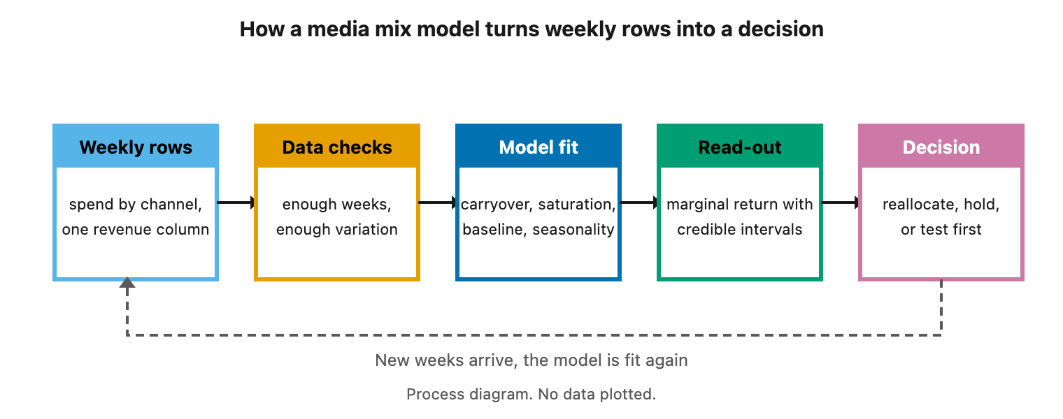
Figure 1. From weekly rows to a decision, with a loop back as new weeks arrive. A process diagram with no data plotted.
In words, weekly revenue is modeled as a baseline plus seasonal movement and promotion effects. To that sum the model adds each channel's transformed spend multiplied by its effect, plus random noise. The fit chooses the effect sizes, carryover rates and curve shapes that best reproduce the observed weeks. Because these pieces are estimated together, an error in one of them can leak into the others.
Each stage has a shorter article behind it, and the next four sections summarize them.
Adstock and saturation set when and how much spend counts
Adstock is carryover, meaning that part of this week's spend keeps working in later weeks. Saturation is diminishing returns, meaning that each added dollar in a channel usually works a little less than the one before. Together they describe when spend counts and how much each unit of spend counts.
In 2017, Google researchers Yuxue Jin and colleagues described both effects, which they called carryover and shape effects, and built a Bayesian model around them. Meridian, Robyn and PyMC-Marketing each offer a small menu of functional forms, and geometric decay and Hill or logistic curves are the common choices.
Two practical consequences follow. Credit for a sale may belong to spend from several weeks earlier. A channel that looks excellent on average can also be a poor place for the next dollar. It may sit on the flat part of its curve.
Meridian's documentation adds that curve estimates rest on the observed range of spend, so results that rely on extrapolation deserve caution. The full treatment, with a worked example, is in adstock and saturation explained in plain terms. For a shorter, plainer take on the whole idea, see What a marketing mix model is in five sentences.
What changes when a model is Bayesian?
A Bayesian MMM states its assumptions as priors, updates them with your data, and returns a distribution for every quantity. For a reader, the main change is the interval: a credible interval is a probability statement about the quantity, given the model and the prior. Other approaches place comparable judgment elsewhere.
Meridian's documentation says a Bayesian regression model combines prior knowledge with signals learned from data. When the data carries little information, the posterior leans on the prior, and when it carries a lot, the posterior leans on the data.
This has a practical edge. Jin and colleagues found that priors significantly influence results with smaller samples and can cause bias. A prior is therefore an input worth reading, not a footnote. Priors can also come from experiments. In 2024, Yingxiang Zhang and colleagues at Google showed how, and reported in simulation that this decreases bias and uncertainty.
Two articles cover this ground. Bayesian vs frequentist MMM compares what each approach shows the reader. Priors in a Bayesian marketing mix model explains how to read and test one.
The model separates revenue into media and non-media parts
An MMM divides revenue into a baseline, seasonal movement, promotions and other controls, and the media channels. Only the media part is credited to channels, so the quality of that split determines how far you can trust every channel figure downstream.
Meridian's control-variable documentation defines baseline outcome as the expected outcome when each treatment variable is set to its baseline value. It says confounders, meaning variables that affect both spend and outcome, should be included to debias causal estimates. Robyn's documentation says it uses Prophet to decompose trend, seasonality, holidays and weekdays.
The split matters because of timing. Suppose revenue peaks every November and you also spend more in November. A model with no seasonal term may credit the whole peak to media. The result looks like a strong channel and behaves like a weak one once you fund it.
Baseline share summarizes the split. A very low value implies that revenue would collapse without marketing. A very high one implies that media does almost nothing. Both deserve a second look. The details are in baseline, seasonality and promotions.
What does an MMM give you?
An MMM gives you three families of output: channel contribution over the fitted period, a response curve for each channel, and marginal return by channel. The third is the most useful for decisions, because it estimates what the next dollar will do. Each should carry a credible interval.
Meridian's documentation distinguishes these clearly. It defines return on investment as the incremental outcome at historical spend divided by spend, a backward-looking grade. Marginal ROI is the return on the next dollar above the historical budget level, which is forward-looking. A marginal ROI well below ROI means the channel is starting to saturate.
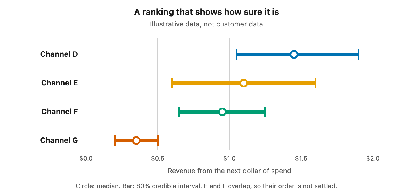
Figure 2. A ranking that shows how sure it is. Illustrative numbers, not real customer data.
The figure shows what a defensible ranking looks like. Channel D is probably strongest and Channel G is clearly weakest. Channels E and F overlap, so their order is unsettled, and no reallocation between them should be presented as a finding.
A small calculation shows why the third output matters. In the illustrative table from the marginal-return article, Channel A returns $2.53 per dollar on average but only $0.40 on its next dollar. Channel B returns $1.18 on average and $0.91 on its next.
Suppose you moved $10 thousand a week from A to B. It would give up about $4.0 thousand and gain about $9.1 thousand. The net is roughly $5.1 thousand. Those numbers are synthetic, and the approximation holds only for small moves. Even so, the arithmetic explains why a report that stops at average return can point in the wrong direction.
That is the argument of marginal ROAS vs average ROAS. The two ratios can rank the same channels in opposite order, and only one of them says where the next dollar should go. A plainer version lives in The handful of numbers worth watching.
How much should you trust the answer?
Trust an MMM to the degree that it shows its work. Look for intervals on every figure, stated priors, convergence diagnostics, an out-of-sample check and, ideally, agreement with an experiment. A model that always returns an answer gives no evidence that the answer is sound, so the ability to refuse is part of the evidence.
Five tests cover most of the ground, and most have an outside reference.
Intervals. A figure with no interval hides how sure the model is. A wide interval is information, and it is often the most honest thing on the page.
Convergence. A Bayesian fit runs several chains that must agree. The Stan reference manual notes that Vehtari and colleagues suggest a general R-hat threshold of 1.01. Their 2021 paper in Bayesian Analysis showed that the older R-hat can miss failures when chains have heavy tails or unequal variances.
Extrapolation. Meridian's documentation says estimating marginal ROI requires extrapolating beyond historical spend, and that uncertainty grows with distance from observed data. Small steps stay inside the evidence.
Experiments. A holdout or geo test is the strongest outside check. Robyn supports calibrating a model with sales and geo experiments, and the 2024 Zhang paper shows one way to do it in a Bayesian model.
Refusal. A model should be able to decline a fit it cannot defend. When the decomposition contradicts itself, or the data cannot separate channels from baseline, the honest output is a reason and not a number.
Refit on a schedule so the estimates stay current
An MMM describes the weeks it was given, so it goes stale as new weeks arrive, budgets move and markets change. Refitting on a schedule keeps the estimates current, tightens intervals as data accumulates, and lets you compare what the last fit predicted with what happened.
Michael Kaminsky of Recast, a vendor of weekly refits, argued in 2023 for weekly refreshes. He said they avoid end-of-quarter surprises and create feedback loops for verifying the model. Meta's Robyn documentation describes a refresh function for monthly, weekly or even daily updates, and it warns that the feature is not yet tested thoroughly.
Each refit should repeat the data checks and convergence checks. It should also be allowed to fail, because a refit that always succeeds may be hiding problems. In a synthetic backtest in that article, refitting every four weeks after a market shift cut forecast error from 17.7% to 14.8%. The refit still lagged the true change. I cover cadence and design choices in how often to refit a marketing mix model.
Three failures that stay quiet
Some failures give no visible sign. The model converges, the intervals look tight and the report looks finished, yet the decomposition is wrong. The usual causes are too little history, channels that move together, a missing promotion, or spend that never varies.
Seasonality credited to media. If the model cannot see the calendar, media inherits the peak. A full year of history, plus the events that moved revenue, prevents most of this.
Confounded channels. When two channels rise and fall together, the data cannot say which one worked, a problem Chan and Perry describe under correlated input variables. Independent budget variation is the remedy.
A prior doing the work. With thin data, results lean on assumptions. The check is to refit with a looser prior and see whether the ranking survives.
None of these is a reason to avoid modeling. Each is a reason to read a model report the way you would read an audit. Look at what it found and at what it could not settle.
Ten questions to ask of any MMM report
The questions below fit on a card and work for any tool or vendor. A good report answers most of them on the page, and the rest can be settled in a conversation with whoever built the model.
- What outcome is being modeled, and does it reconcile to your ledger?
- How many weeks of data are there, and do they include a full year?
- Does each channel's spend vary enough to be separated from the baseline?
- Are carryover and saturation estimated per channel, with intervals?
- What is the baseline share, and does it pass common sense?
- Which priors were used, and where did they come from?
- Do the marginal returns carry credible intervals, and do adjacent ones overlap?
- How was the fit checked, both on convergence and on held-out weeks?
- Has any experiment confirmed or contradicted the model?
- When is the next refit, and what would change the recommendation?
The order is deliberate. The early questions concern data and can be answered before any modeling. The later ones concern evidence, and they decide how firmly you can use the output.
Frequently asked questions
What is the difference between MMM and attribution?
Attribution assigns credit to individual touchpoints along customer journeys. An MMM works with aggregate weekly spend and revenue and estimates each channel's incremental contribution. They answer different questions, and many teams use both. Neither one replaces the other, and each can inform the assumptions behind the other.
How much data does an MMM need?
It needs enough weeks to see seasonality and enough variation in spend to separate channels. A yearly cycle cannot be estimated from less than a year of weekly data, and seeing it repeat takes longer. Below that, seasonality can tangle with trend, so intervals should be wide and results treated as directional.
Does an MMM replace experiments?
No. An MMM estimates effects from historical variation, while an experiment measures the effect of one change directly. They complement each other. Experiment results can calibrate a model, either as priors or as checks, and a model can suggest which experiments are worth running next.
Can I trust a marginal return outside my usual spend range?
Only with caution. Meridian's documentation warns that estimates beyond historical spend require extrapolation, and that uncertainty grows with distance. Move budget in small steps, refit after each move, and confirm any large change with a test before you commit to it fully.
How often should I refit?
Match the cadence to your decisions. Recast advocates weekly refreshes, and Robyn supports monthly, weekly or daily ones. A reasonable rule is to refit at least as often as you reallocate budget, and to make sure every refit runs its checks. That rule is mine, not a published standard.
Where to go next
To see these ideas applied to your own weekly rows, join the waitlist at bayesin.com/request-access. Bayesin checks your data before it fits. It blocks a fit below 52 weeks, recommends 104, and warns when a channel's spend varies by less than 15% of its average. It also refuses fits it cannot defend and shows a credible interval on every figure.
Sources
Every external claim above comes from the pages listed here, each opened on the retrieval date shown. Statements about Bayesin come from its own code and site content, not from these sources.
- Google for Developers, "About the project," Meridian documentation, living document, accessed 2026-09-18 (retrieved 2026-09-18)
- Google for Developers, "Bayesian Inference in Meridian," Meridian documentation, living document, accessed 2026-09-18 (retrieved 2026-09-18)
- Google for Developers, "Incremental Outcome, ROI, mROI & Response Curves," Meridian documentation, living document, accessed 2026-09-18 (retrieved 2026-09-18)
- Google for Developers, "Control variables," Meridian documentation, living document, accessed 2026-09-18 (retrieved 2026-09-18)
- Google for Developers, "Media saturation and lagging," Meridian documentation, living document, accessed 2026-09-18 (retrieved 2026-09-18)
- Google Research, Jin, Wang, Sun, Chan and Koehler, "Bayesian Methods for Media Mix Modeling with Carryover and Shape Effects", 2017 (retrieved 2026-09-18)
- Google Research, Sun, Wang, Jin, Chan and Koehler, "Geo-level Bayesian Hierarchical Media Mix Modeling", 2017 (retrieved 2026-09-18)
- Google Research, Chan and Perry, "Challenges and Opportunities in Media Mix Modeling", 2017; section headings 4.1.1, 4.1.2, 4.1.3 and 4.2 read in the full text (retrieved 2026-09-18)
- Google Research, Zhang et al., "Media Mix Model Calibration With Bayesian Priors", 2024 (retrieved 2026-09-18)
- PyMC-Marketing, "Guide to Adstock Transformations", living document, accessed 2026-09-18 (retrieved 2026-09-18)
- Meta, "Key Features," Robyn documentation, living document, accessed 2026-09-18 (retrieved 2026-09-18)
- Stan Development Team, "Stan Reference Manual: Posterior Analysis", living document, accessed 2026-09-18 (retrieved 2026-09-18)
- Vehtari, Gelman, Simpson, Carpenter and Bürkner, "Rank-normalization, folding, and localization: An improved R-hat for assessing convergence of MCMC," Bayesian Analysis, 2021 (retrieved 2026-09-18)
- Recast, Kaminsky, "Why should we refresh our MMM every week?", 2023 (retrieved 2026-09-18)
See it on your own rows.
Bayesin is pre-launch. Join the waitlist and we will reach out as access opens.
Get new posts by email.
New posts only. See privacy for what we keep.