B2B
Testing when you sell to accounts
Testing when you sell to accounts: account-level and regional holdouts compared on one synthetic list, with detectable effect, expected effect and power.
Brandon Cade · Nov 17, 2026 · 12 min read
Key Takeaways
- Randomize accounts where you can target them, and regions where you can't.
- On a synthetic 2,400-account list, an account split detects 2.72 points on a 6% base, and a regional split needs 4.91.
- The effect I'd expect is about 1 point.
- So plan to narrow a range, not to get a verdict.
On a list of 2,400 target accounts, the smallest closed-won effect a test can reliably find is larger than the base rate itself. That's 1.25 points on a base of 1.2%, in the synthetic list I use here.
That doesn't make testing pointless, but it does change what you plan for. This post shows you how to pick a unit, size the test and choose what to read. It also shows what to do when the likely answer is a range. Every number below comes from settings I chose for this example, so none of it is customer data or a benchmark. The designs are a method you can run on your own list, not a list of what Bayesin supports. If you want the basics first, start with what a holdout test is.
Why is the account the unit?
Assign the account, because one buying decision spans many people. Digital Commerce 360's 2026 report on Forrester's research puts the average at about 13 internal stakeholders, plus nine external. That's a secondary report of a paid study, so treat the number as directional.
If contacts from one account sit in both arms, your control group hears about the ads from colleagues. The comparison then shrinks toward zero, and nothing in the read tells you it did. Research at LinkedIn shows the same kind of problem in a different setting. In 2017, Saveski and colleagues found network effects and bias in standard A/B tests on LinkedIn's own platform. Those were product experiments rather than ads, so take it as an analogy.
Clustering also has to match how you assign. Abadie, Athey, Imbens and Wooldridge argue that adjusting for clusters matters when assignment is correlated with cluster membership. If you assign whole accounts or whole regions, analyze them that way.
Before you randomize, group parent and child companies. Otherwise one buying committee can land in both arms under two names. This is far easier to fix now than after the read.
Which designs can your channels support?
The channel decides the unit, because you can only hold out what you can target. The table below is my reading of where each channel usually lands, so check it against your own setup.
- LinkedIn and other list-targeted channels: Usual unit: Account; What to check: Can you exclude a company list?
- Paid search, YouTube: Usual unit: Region; What to check: Can spend be set by region?
- National buys: Usual unit: Neither; What to check: Use a national spend pulse
LinkedIn's rules set a floor for list tests. Its company list help page asks for at least 300 rows and recommends 1,000 or more. A list must also match at least 300 member accounts to run in an active ad set. The page doesn't cover exclusion lists, so confirm that before you plan around one.
LinkedIn also runs its own lift product. Its methodology page asks for at least 10 conversions in each group. It moved to Bayesian lift probability in June 2026, and it labels 90% or more as "Lift Detected". The page adds that "conclusive results aren't guaranteed". It doesn't explain how members are assigned, and LinkedIn's 2025 marketing post says only that groups are randomized.
So a member-level split may put contacts from one account on both sides, and it's worth asking. These pages can change, so check the current versions before you rely on them. Lift probability is LinkedIn's own measure, so don't read it as a credible interval. For more, see reading a platform lift study.
Regions come from a longer tradition. Vaver and Koehler at Google set out the geo design in 2011, with non-overlapping regions randomized to treatment and control. Kerman, Wang and Vaver added a time-based regression for few units in 2017. I cover how to match regions separately.
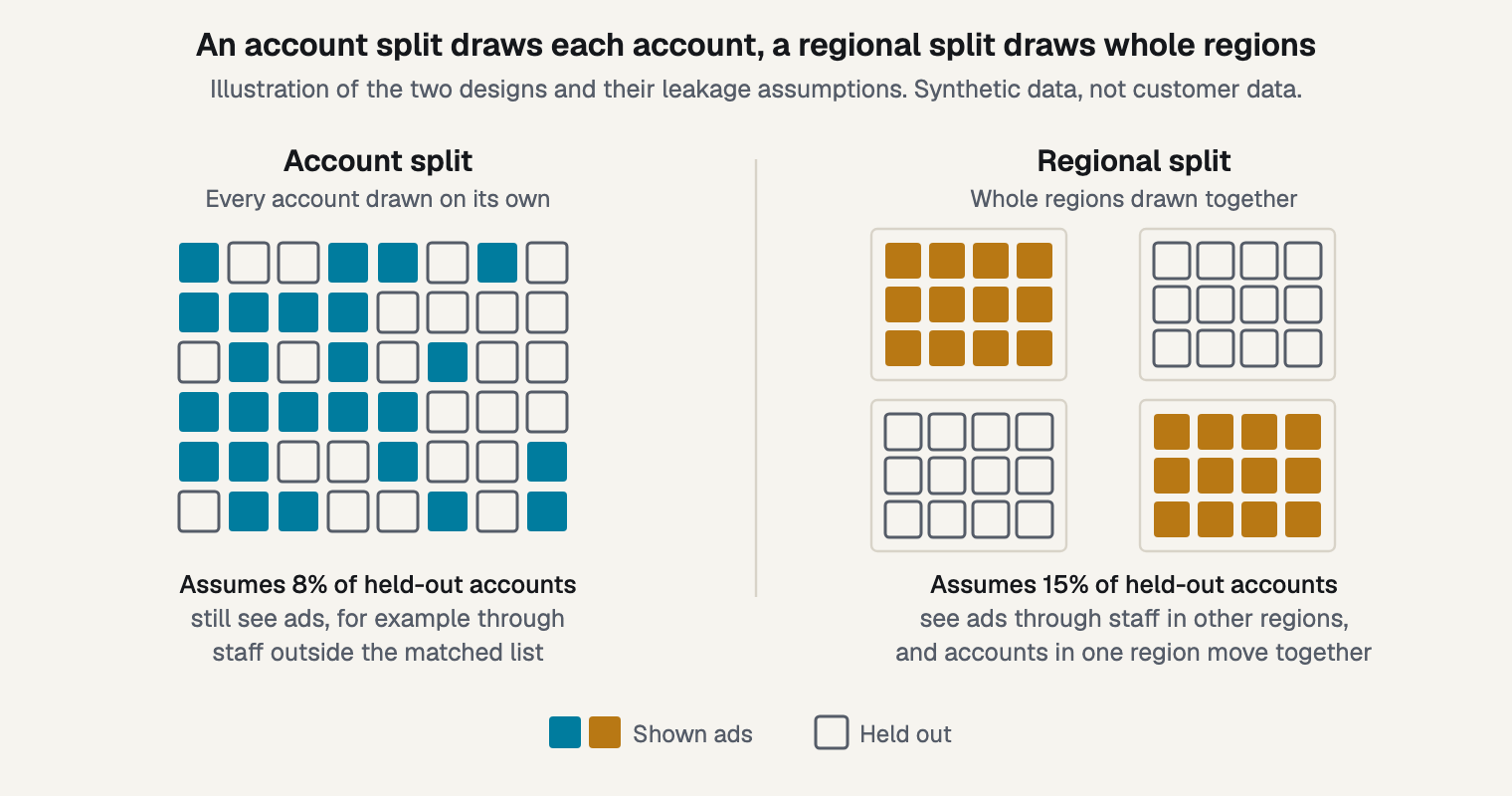
Figure 1. The two ways to split a list, with the leakage I assume for each.
How do the two designs compare on one list?
On this list, accounts detect a smaller effect at every correlation I ran. Even with no correlation between regions at all, regions would need 2.84 points against 2.72, because 12 regions a side need a wider multiplier.
The list. It has 2,400 accounts in 24 equal regions, read over 26 weeks. An account opens an opportunity with probability 6.0% and closes won with probability 1.2%. Spend on the list is $30,000 a week, opportunities average $85,000, and I assume $3.00 of incremental pipeline per $1. Ads reach 70% of treated accounts. They also reach 8% of control accounts in the account design, and 15% in the regional one, through staff elsewhere. These are my assumptions, and none is typical of anything.
The expected effect. The treated half gets $390,000 of spend, which at $3.00 is $1,170,000 of pipeline. That's 13.8 opportunities on 1,200 accounts, or 1.15 points. Leakage reduces it to 1.02 points on accounts and 0.90 on regions.
Detectable effect is what the design can reliably find, and it differs from what you expect the channel to do. These are frequentist design calculations: 2.8 x standard error at 5% two-sided and 80% power, as in how to size a test. Regions use 2.93, because 22 degrees of freedom call for t values.
Design effect is the correction for accounts in one region moving together, since regional data holds less information than its count suggests. Killip, Mahfoud and Pearce give the correction, 1 + (m - 1) x ICC. Here m is accounts per region and ICC is the intracluster correlation. They report that ICC is usually about 0.01 to 0.02 in human studies, though that's primary care research. Estimate yours from your pre-period.
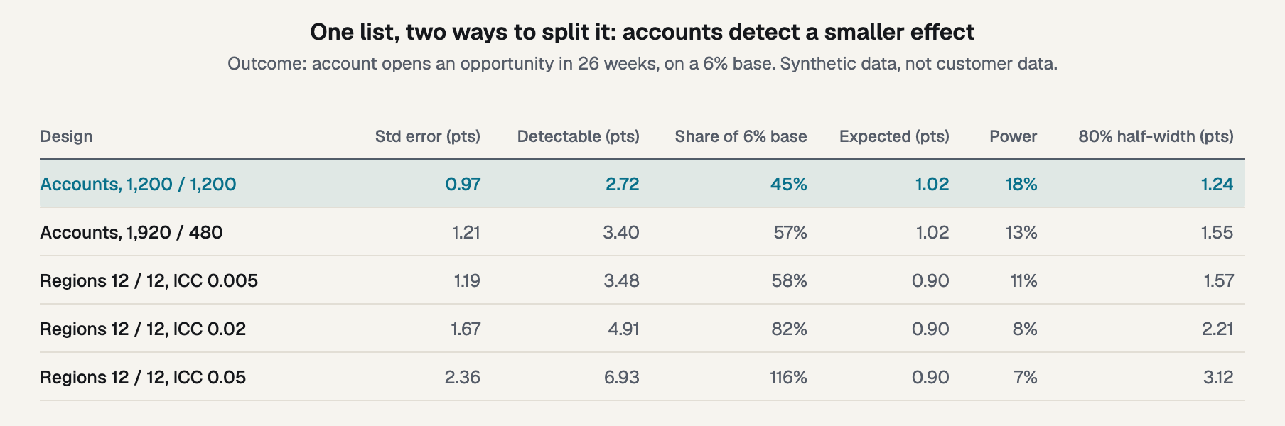
Figure 2. One list run through five designs.
An even account split detects 2.72 points, or 45% of the 6% base, while regions at an ICC of 0.02 need 4.91 points, or 82%. At that ICC the design effect is 2.98, so 2,400 accounts carry the information of about 805. At 0.005 and 0.05 the effective counts are 1,605 and 403.
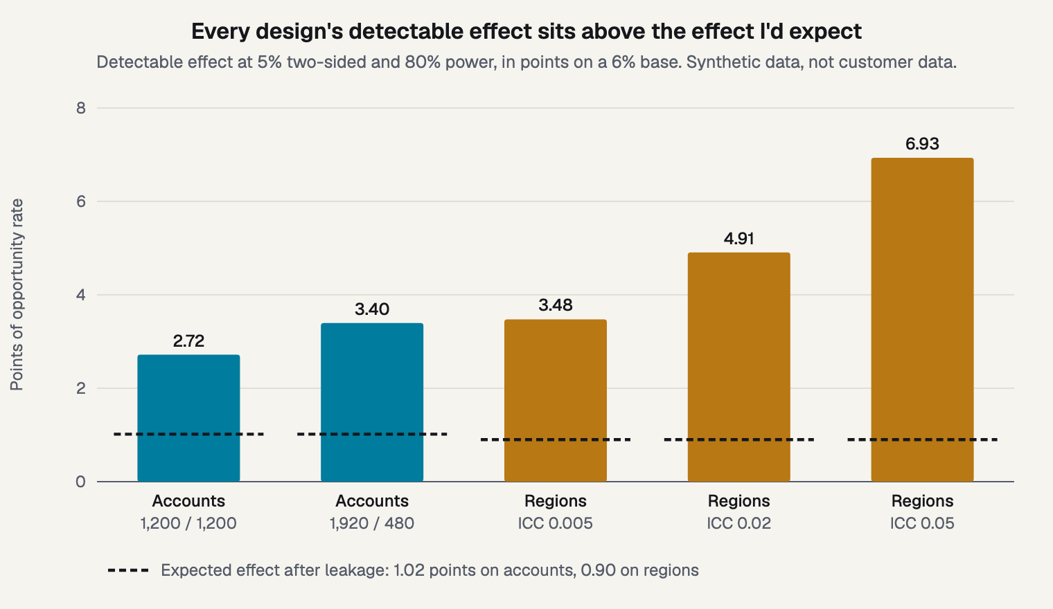
Figure 3. Every detectable effect is more than 2.5 times the effect I expect.
I checked the formulas with 20,000 simulated runs of each design. The spread of the difference came out 1% to 4% above the standard error, because the treated arm has a higher rate. Power came out at 17%, 11%, 11%, 8% and 6%, against 18%, 13%, 11%, 8% and 7% from the formulas. The largest gap is the 80/20 split, where the pooled test runs a little conservative.
The table flatters regions in one way, because it assumes equal sizes. Real territories differ, and Eldridge, Ashby and Kerry treat that adjustment for unequal clusters. Rep coverage can differ by region too, which is my reasoning and not a sourced result.
A regional test can still be the right one. If you can't exclude accounts on a channel, the 2.72 isn't on offer, and the honest comparison is 4.91 against no test at all.
What if your expected effect is below the detectable effect?
Then the test narrows a range rather than delivering a verdict. Here the expected effect is 1.02 points, the detectable effect is 2.72, and power is 18%. Power is a frequentist quantity: the chance of a two-sided 5% rejection if the true effect is the expected one.
Reaching 80% power at 1.02 points would take about 8,600 accounts per arm, roughly seven times this list. Lewis and Rao show this is hard even at scale. In 25 experiments across retail and brokerage, the median interval on return was over 100 percentage points wide.
This supports part of a fair objection. Dreamdata argues that incrementality measurement is typically useful above $1 million a month, and that smaller B2B teams are better served by attribution. On a yes-or-no question, my table agrees with them.
I'd ask a different question, though: how much does the test narrow what you already believe? An 80% half-width on the even account split is 1.24 points. With a weak prior and a normal approximation, an 80% credible interval has about that half-width. It means that, given the model and prior, the effect likely sits in that range, as I cover in how to read a credible interval. It isn't power, and it isn't a chance that the test will find anything.
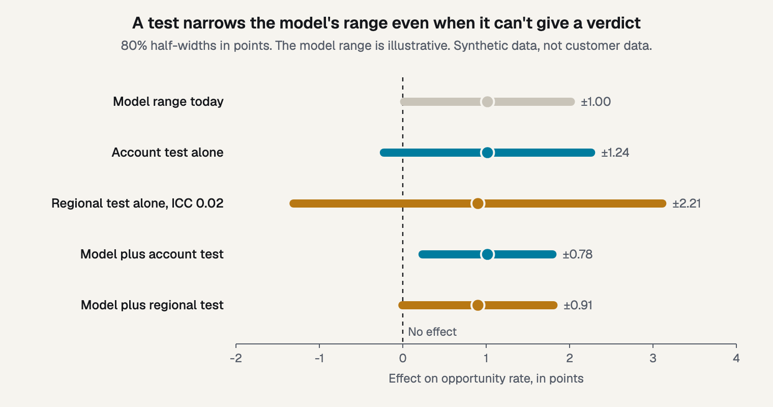
Figure 4. Combining a test with an illustrative model range narrows it, more with accounts than regions.
Suppose your model's 80% range is plus or minus 1.00 points, which is a number I made up to show the method. Combining it with the account test gives plus or minus 0.78, or 22% narrower. The regional test at an ICC of 0.02 gives 0.91, or 9% narrower. That treats the two sources as independent and Normal, so read it as a planning number.
The account test helps even with a half-width wider than the model's range, because independent evidence adds up. Still, 9% may not justify the cost, so compare it with what a test costs. If the interval crosses zero, that's still useful, as long as you planned for it.
If you want a sharper read, you have five levers:
- Concentrate spend on the treated arm.
- Lengthen the window.
- Make a bigger change.
- Widen the list.
- Accept a range, and say so before you start.
Which outcome do you read, and when?
Read opportunities first, because closed-won arrives too late and too sparse on most lists. On this list it comes to 14.4 wins per arm in the window, so the first read would have little to work with.
- Account opens an opportunity: Detectable effect: 2.72 points; Share of base: 45%
- Pipeline dollars: Detectable effect: Not in points; Share of base: 85%
- Account closes won: Detectable effect: 1.25 points; Share of base: 104%
Counts beat dollars on the same accounts. Suppose deal size is lognormal with a sigma of 1.1. Pipeline per account then has a coefficient of variation of 7.41, which takes the relative detectable effect from 45% to 85%. That's the same order as the coefficient of variation of 10 that Lewis and Rao call common, though their setting is retail and brokerage.
Using opportunities as a stand-in carries a condition. Athey, Chetty, Imbens and Kang set it out for surrogates: the treatment's effect on the long-term outcome has to pass through the stand-in. If a channel brings more opportunities that close less often, opens will flatter it. Their setting is a job-training experiment, so this is an analogy.
The window has to allow for the lag, and I cover how long a test should run in detail. Vendor guidance differs here. Abmatic says one sales cycle plus a buffer, while Single Grain says 8 to 12 weeks for B2B with longer cycles. Report closed-won later as a second read, and don't claim it was powered.
How do you make the test sharper?
Pair or stratify before you randomize, and use the pre-period afterward. Imai, King and Nall argue that pairing should be used "whenever feasible" in cluster-randomized work. For accounts, pair on size, segment and prior pipeline.
Pre-period data helps after the test. Deng, Xu, Kohavi and Walker cut variance by about 50% at Bing, which isn't a B2B list. So I assumed less here. If prior-year pipeline explains 30% of the variance, the standard error falls from 0.97 to 0.81 points. The detectable effect falls to 2.27 points and power rises from 18% to 24%.
That helps, but it doesn't change the conclusion. Lock the plan before the start, including the outcome and read date, and don't stop early because a number looks good.
Frequently asked questions
How many accounts do I need?
It depends on your base rate and the effect you expect, so compute it. A common vendor rule, Abmatic's 200-plus accounts per cohort, is written for a 60-day window. On this list's 6% base, 200 per arm has a detectable effect of 6.65 points, or 111% of base.
Should the holdout be 50/50?
A 50/50 split gives the smallest detectable effect, at 2.72 points here. An 80/20 split detects 3.40 points and leaves fewer accounts dark, so you forgo less exposure. On closed-won it leaves only 5.8 expected wins in the smaller arm. Choose by what the lost exposure costs you.
Can I test contacts instead of accounts?
Only if colleagues can't influence each other, which is rare on a buying committee. A contact split looks larger on paper because the count is higher. But if contacts in one account land in both arms, the control is exposed, and the read shrinks toward zero without warning you.
Who runs the test?
Your team does. Where the model knows least, Bayesin designs the test, and your team runs it, while Bayesin tracks it and reads the result. Bayesin never changes spend. The account and regional designs here are general method, and you can run them on your own list without any particular tool.
Start with your own list
Take your target list this week and compute three numbers: your base rate, the detectable effect at your count, and the effect you expect. If the expected effect is below the detectable one, write down how far the test would narrow your range. Then decide whether that's worth its cost.
Sources
- The Annals of Family Medicine, "What Is an Intracluster Correlation Coefficient? Crucial Concepts for Primary Care Researchers," Killip, Mahfoud and Pearce, 2004
- International Journal of Epidemiology, "Sample size for cluster randomized trials: effect of coefficient of variation of cluster size and analysis method," Eldridge, Ashby and Kerry, 2006
- Statistical Science, "The Essential Role of Pair Matching in Cluster-Randomized Experiments, with Application to the Mexican Universal Health Insurance Evaluation," Imai, King and Nall, 2009
- arXiv, "When Should You Adjust Standard Errors for Clustering?," Abadie, Athey, Imbens and Wooldridge, 2017, revised 2022
- KDD, "Detecting Network Effects: Randomizing Over Randomized Experiments," Saveski et al., 2017
- Google Research, "Measuring Ad Effectiveness Using Geo Experiments," Vaver and Koehler, 2011
- Google Research, "Estimating Ad Effectiveness using Geo Experiments in a Time-Based Regression Framework," Kerman, Wang and Vaver, 2017
- Quarterly Journal of Economics, "The Unfavorable Economics of Measuring the Returns to Advertising," Lewis and Rao, 2015
- NBER, "The Surrogate Index," Athey, Chetty, Imbens and Kang, 2019, revised 2024
- WSDM, "Improving the Sensitivity of Online Controlled Experiments by Utilizing Pre-Experiment Data," Deng, Xu, Kohavi and Walker, 2013
- LinkedIn Marketing Solutions Help, "Company list targeting in Campaign Manager," official documentation, 2026
- LinkedIn Marketing Solutions Help, "Brand and Conversion Lift Testing status and methodology," official documentation, 2026
- LinkedIn, "Accelerate Pipeline & Prove ROI with LinkedIn's Newest Ad Innovations," vendor post, 2025
- Digital Commerce 360, "Forrester: B2B buying groups expand as they question AI," secondary report, 2026
- Dreamdata, "Incrementality - Why you need to consider it," vendor page, undated
- Abmatic AI, "Marketing Attribution Lift: Measure Incrementality," vendor post, 2026
- Single Grain, "Incrementality Testing Playbook: Math, Types, Runbook," agency guide, 2026
See it on your own rows.
Bayesin is pre-launch. Join the waitlist and we will reach out as access opens.
Get new posts by email.
New posts only. See privacy for what we keep.