Testing
How big does a marketing test need to be? Power and detectable effect, by hand
How big a marketing test needs to be, worked by hand: measure noise with fake tests, turn it into a detectable effect, and check it against the break-even line.
Brandon Cade · Nov 5, 2026 · 12 min read
Key Takeaways
- Power and detectable effect come from four inputs: noise, weeks, dollars changed and your threshold.
- One synthetic design detects an incremental return of 1.36 at a 95% threshold and 80% power.
- If the true return is 1.3, it has only 30% power to show a channel below a 2.0 break-even.
- Size against your decision line.
In a synthetic test with no effect at all, the chart still shows a lift. Across 20,000 no-effect runs on one synthetic brand, the middle 95% of results ran from -5.0% to +5.2% of holdout revenue. In 22% of runs, the "lift" was 2% or more.
A test too small to read costs real revenue and returns a shrug. You can find that out before you book it, because an incrementality test power analysis needs only a spreadsheet and some past weeks of data.
By the end, you'll have a minimum detectable effect for your own test and know how it compares with your decision. Every number here is synthetic: illustrative, not real customer data. If you're still choosing where to test, start with which channel to test first.
What do power and detectable effect mean?
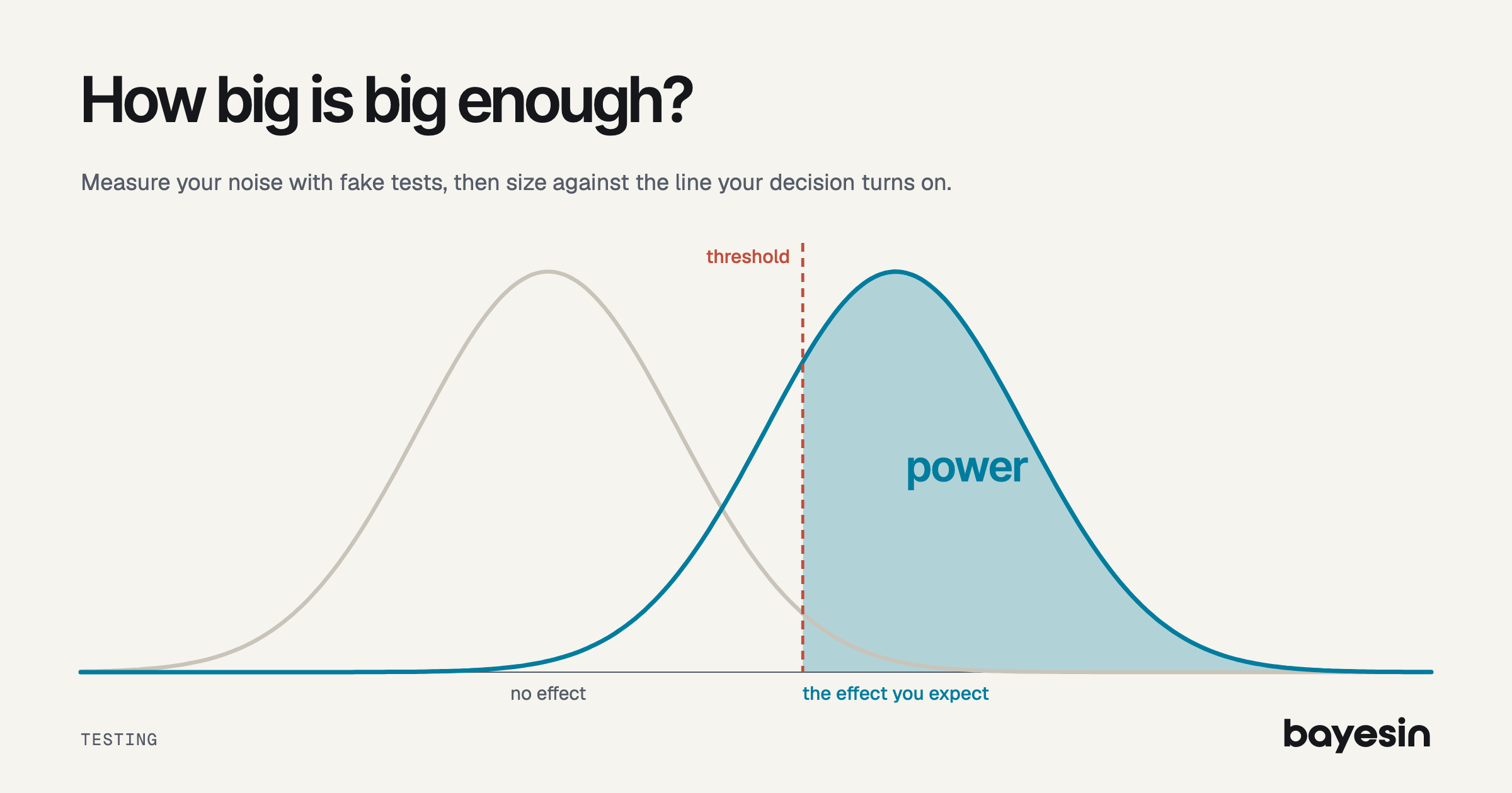
Power is the chance that a test crosses its threshold if an effect of a stated size exists. Minimum detectable effect (MDE) is the effect at which that chance reaches a chosen level, usually 80%.
The MDE describes the design, and it isn't a forecast. A test with an MDE of 1.36 doesn't expect a return of 1.36. It says only that if the true return were 1.36, this design would cross its threshold four times in five. Keep that apart from the expected effect, which comes from what you believe about the channel. Sizing is the act of comparing the two.
The formula is the standard one. NIST's handbook gives sample size as N = (z1 + z2)^2 x (sigma / delta)^2, with one z for the threshold and one for power. Rearranged for the effect, that's delta = (z1 + z2) x sigma / sqrt(N), which gives the rule I use in my testing posts:
Detectable effect = (threshold z + power z) x standard error = (1.96 + 0.84) x standard error = 2.8 x standard error
So for a two-sided 5% threshold and 80% power, the multiplier is 2.8, or 2.802 before rounding. Gelman and Carlin show the same relationship in reverse: a true effect 2.8 standard errors from zero gives 80% power.
Sizing matters because advertising effects are small against sales noise. Lewis and Rao found a median confidence interval on return over 100 percentage points wide across 25 experiments. That's why tests have such wide intervals. Those were user-level tests, while this post uses regions and revenue.
Step 1: How do you measure your noise?
Run fake tests on past weeks, and the error of those fake reads is your noise. Use counterfactual error rather than raw week-to-week swings, because a good comparison group removes much of the swing.
Pick a past stretch with no big changes, pretend the test started, and predict the holdout regions from your other regions. Then compare with what happened, and repeat over many start dates and region draws. Kerman, Wang and Vaver call these pseudo-experiments, and GeoLift's walkthrough simulates on historical data in the same spirit.
Measure the whole read rather than one week, by taking the standard deviation of the 8-week total across your fake tests. Weekly errors are rarely independent, and independence is what sqrt(weeks) assumes. If your weekly figure comes from single-week errors, autocorrelation inflates the standard error like this:
- 0: Standard error inflation over 8 weeks: 1.00x; Detectable return: 1.36
- 0.2: Standard error inflation over 8 weeks: 1.19x; Detectable return: 1.62
- 0.4: Standard error inflation over 8 weeks: 1.43x; Detectable return: 1.95
- 0.6: Standard error inflation over 8 weeks: 1.75x; Detectable return: 2.39
Method matters too. Recast, a vendor in this category, ran 32,000 simulated fits across four open-source tools and reported false positive rates from 3.3% to 30.0%. Rates varied by tool and scenario, and Recast says its data may suit some methods, so read that as directional and test your own setup.
Here's the synthetic brand I'll use from here on. Weekly revenue is $268,000, the channel spends $19,500 a week, and margin is 50%, so break-even return is 2.0. The holdout regions hold 25% of revenue, or $67,000 a week.
The design pauses the channel in those regions for 6 live weeks and reads at week 8. Fake tests show an error equal to 7.5% of holdout revenue per week, or $5,025. The model's 80% credible interval on return is 0.5 to 2.1, with a midpoint of 1.3.
Step 2: How do you turn noise into a detectable effect?
Multiply the standard error by 2.8 for a 95% threshold and 80% power. It takes four steps, and each fits in one spreadsheet cell.
- Noise over the read. $5,025 x sqrt(8) = $14,213.
- Dollars withheld. $19,500 x 0.25 x 6 = $29,250.
- Standard error of return. $14,213 / $29,250 = 0.486.
- Detectable effect. 2.802 x $14,213 = $39,819. That's 7.4% of the $536,000 of holdout revenue over 8 weeks, or an incremental return of 1.36.
Rounding the multiplier to 2.8 gives $39,796 and the same 1.36. In a spreadsheet, the whole calculation is one line:
= (NORM.S.INV(0.975) + NORM.S.INV(0.8)) * weekly_error * SQRT(read_weeks) / dollars_withheld
Your threshold is a choice. With an 80% interval as the threshold, the multiplier is 1.28 + 0.84 = 2.12, and the detectable return falls from 1.36 to 1.03. That isn't free, however. One in five no-effect tests will exclude zero, half of them positive, so 1 in 10 shows positive lift from noise alone. At the 95% threshold, it's 1 in 40.
Step 3: Is that small enough for your decision?
Compare the detectable effect with the effect you expect, and with the line your decision turns on. Zero is usually not that line.
Start with zero: the model's midpoint is 1.3, a little below the 1.36 this design can detect. If the true return is 1.3, this test has 76% power against zero, and at 0.6 it has 23%. Low power also comes with overstatement, which Gelman and Carlin measure as exaggeration: the average size of estimates that cross, divided by the true effect. Here it's 2.06x at 0.6 and 1.15x at 1.3, and it reaches 1.13x at 2.8 standard errors.
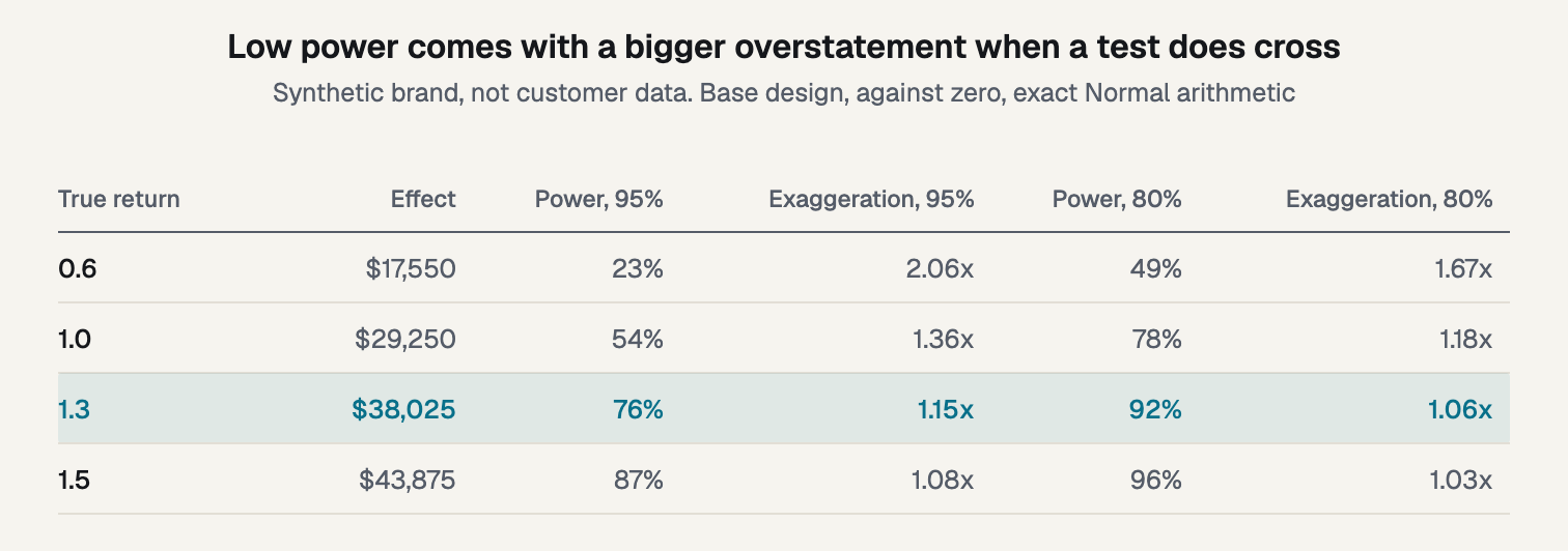
Figure 1. Power and exaggeration at four true returns, against zero.
Your decision probably isn't whether the return is above zero, because with a 50% margin, it's whether the return is above 2.0. The gap between 1.3 and 2.0 is 0.7, which is only 1.44 standard errors. At a true 1.3, the chance of showing it below 2.0 is 30% at the 95% threshold and 56% at an 80% interval.
The design that reads well against zero reads poorly against break-even. Getting 80% power on that 0.7 gap needs a standard error of 0.25, which is about 3.8 times the information in the current read.
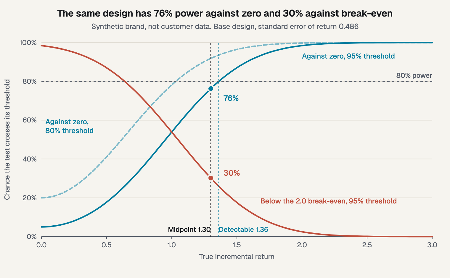
Figure 2. One design, two questions: 76% power against zero and 30% against break-even.
Take the expected effect from the model's interval or outside evidence, and hold it loosely. Gelman and Carlin warn that effect sizes from small earlier studies tend to run high. Korkames, Stanley and Stremersch report bias-corrected advertising elasticity of 0.0008 short term and 0.03 long term, across 538 elasticities. Those are elasticities rather than returns, so they support caution and not a planning value.
If your expected effect sits below the MDE, your power is under 80%. Below 1.96 standard errors, a return of 0.95 here, a miss is more likely than a detection. Measured gives a similar vendor rule: if a test can't detect a decision-changing lift, redesign it.
What does a fake lift look like?
It looks like a real one. Noise alone produces results that cross thresholds at a known rate, and low-power tests that do cross overstate the effect.
I built a synthetic brand to show this: 30 regions over 104 weeks, with lognormal region sizes and total weekly revenue averaging $268,000. Revenue has a yearly season, a shared weekly shock and a region weekly shock. Weekly shocks are autocorrelated at 0.4, and region shocks are 9.01%.
Each of 20,000 seeded runs draws a new history and picks a start week after week 52. It then assigns regions at random until they hold about 25% of revenue. Next it fits a holdout-to-control ratio on the prior 52 weeks and predicts the 8 test weeks. There's no channel effect at all.
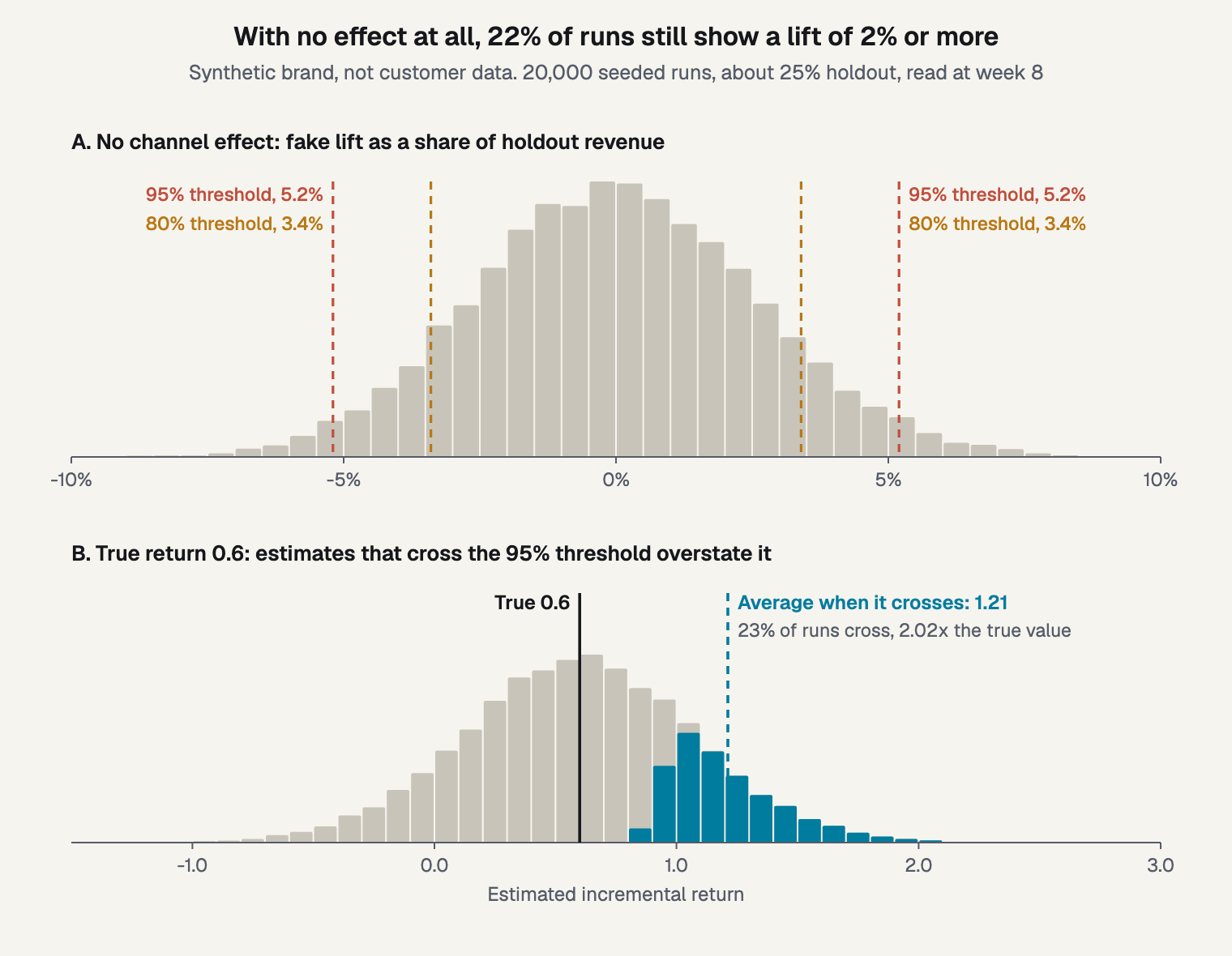
Figure 3. Fake lift with no effect, and estimates at a true return of 0.6.
The read noise across runs was $14,024, within 1.3% of the hand calculation's $14,213. That's by design, since I tuned the shocks to match. What I didn't tune is how often each way of setting the standard error raises a false alarm:
- Weekly error x sqrt(8): Median: $8,804; Crossed 95% (nominal 5%): 21.3%; Crossed 80% (nominal 20%): 41.1%
- Same regions, rolling 8-week windows: Median: $13,026; Crossed 95% (nominal 5%): 9.1%; Crossed 80% (nominal 20%): 23.8%
- 60 fake tests with fresh regions: Median: $13,700; Crossed 95% (nominal 5%): 6.2%; Crossed 80% (nominal 20%): 20.6%
- True noise across all runs: Median: $14,024; Crossed 95% (nominal 5%): 5.2%; Crossed 80% (nominal 20%): 19.3%
The first row is the warning. Single-week errors times sqrt(8) understate the true noise by 1.59x, so false alarms run at 21.3% against a nominal 5%. Autocorrelation explains 1.43x of that, and error in the fitted ratio takes it to about 1.55x.
The second row looks fine on the median, but it swings. With only 52 weeks to roll through, its standard error ranged from $8,774 to $18,786 between the 10th and 90th percentile. Shuffling regions as well narrows that to $11,339 to $16,523, and false alarms fall to 6.2%. In this setup, that's the placebo I'd use.
Now add a known effect. At a true return of 0.6, 23.4% of runs crossed the 95% threshold, against 23.5% in the exact table. Those runs averaged an estimate of 1.21, which is 2.02x the true value, against 2.06x exact. No crossing run reported less than 0.82, so none could report the truth. At a true return of 1.3, power was 77.0% against 76.3% exact, and exaggeration was 1.14x against 1.15x.
Which lever should you pull?
Change more dollars, run more live weeks, or reduce noise. Holdout share may help less than you'd expect, and a smaller cut hurts more than you'd expect.
Cutting spend by half instead of pausing doubles the detectable return, from 1.36 to 2.72. Moving from 6 to 12 live weeks takes it to 0.90, at twice the withheld dollars. Reducing noise from 7.5% to 5% takes it to 0.91 with no extra dollars. Only three of the seven designs fall below the model's midpoint of 1.3.
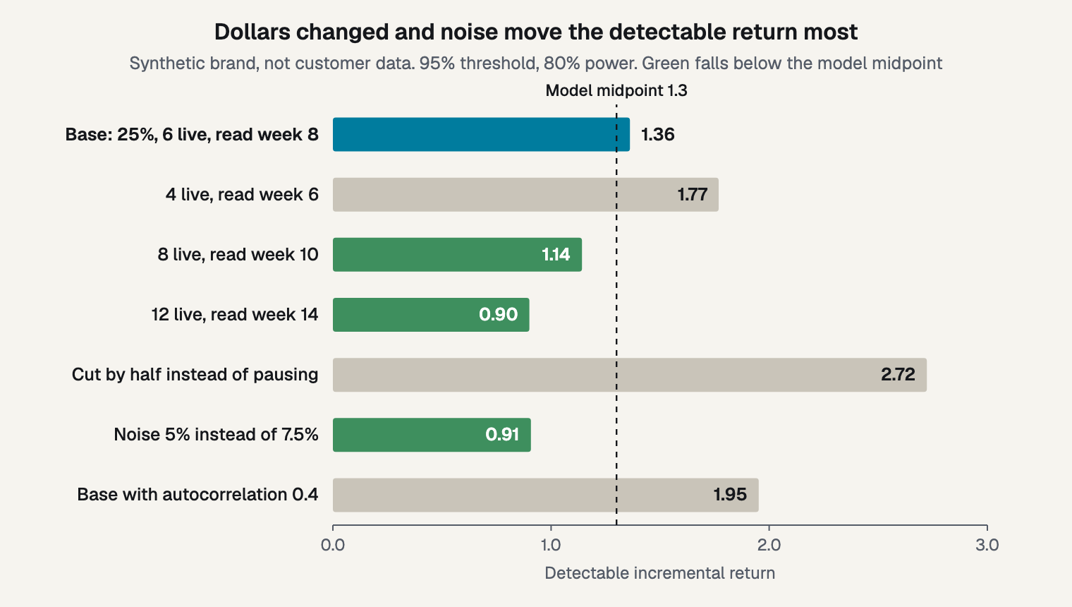
Figure 4. What each design change does to the detectable return.
Holdout share is the surprise. If percentage noise doesn't change with group size, a larger holdout costs more without improving the detectable return, since dollars and noise rise together. In real data, smaller groups are noisier, so the truth usually falls between these two columns:
- 10%: Dollars withheld: $11,700; Noise share stays 7.5%: 1.36; Noise grows as regions shrink: 2.15
- 25%: Dollars withheld: $29,250; Noise share stays 7.5%: 1.36; Noise grows as regions shrink: 1.36
- 40%: Dollars withheld: $46,800; Noise share stays 7.5%: 1.36; Noise grows as regions shrink: 1.08
So measure it, by running your placebo tests at each candidate share to see which column you're in. Each lever also has a cost, in revenue or calendar time.
Two limits apply: it treats the effect as proportional to dollars and as fully captured in the read window, and carryover shrinks the captured share. Changing dollars is also how you start adding variation to a flat channel, and a scale-up reads spend you haven't tried, where the range widens.
How does this read for a Bayesian test?
The same planning works, but say what you mean. Power is a long-run frequentist idea, and a Bayesian plan reports assurance and expected interval width instead.
Power, MDE and false positive rate describe a procedure under repeated tests. A frequentist read reports a confidence interval and a Bayesian read reports a credible interval, as I cover under confidence and credible intervals. A credible interval isn't a hypothesis test. It holds the true value at the stated probability given the model and prior, which is what a credible interval says and no more. "Excludes zero" lines up with a frequentist test only under a flat prior.
Two planning numbers carry over. Assurance, as Kunzmann and colleagues review it, averages power over a prior. Using the model's interval as the prior, with mean 1.3 and standard deviation 0.624, assurance is 67% at the 95% threshold. Power at the midpoint alone was 76%, so uncertainty about the effect costs nine points.
The second needs no threshold: expected width. The standard deviation falls from 0.624 to 0.383, so the 80% interval narrows from 1.60 to 0.98, or 39%. Kerman and colleagues call a credible interval's half-width its precision and find it more concrete than power, so I'd plan on that number.
Frequently asked questions
What is a good minimum detectable effect?
One smaller than the effect your decision turns on. Vendor figures like 2% to 5% lift, as Measured cites for a well-powered geo test, aren't a standard, since they depend on noise and design. In my synthetic example, 7.4% of holdout revenue came close against zero and fell well short against break-even.
What if the MDE is bigger than the effect I expect?
Change more dollars, run longer, reduce noise or choose another test. If none of those work, the honest result is that this test can't answer this question at a price you'd pay. That's a useful thing to learn before the money goes out, and worth recording.
Should I use a 95% or an 80% threshold?
Choose before the test starts, and accept the false alarm rate that comes with it. At a 95% threshold, 1 in 40 no-effect tests shows positive lift. At an 80% interval, it's 1 in 10. A cheap, reversible decision can live with the second, and a large one usually can't.
Can I calculate power after the test?
Not to explain a null. Observed power follows directly from the p value, so it tells you nothing the result didn't, as Hoenig and Heisey show. Use the interval instead. It shows which effect sizes the test leaves open, and you can compare those with your decision line directly.
What to do before you book the test
Run the sheet on your own numbers before you book the test. Three steps cover it:
- Measure noise with fake tests on past weeks, reading the whole window.
- Calculate the detectable effect with the 2.8 multiplier.
- Compare it with your decision line, not only with zero.
Bayesin designs and reads tests. Your team runs them, and Bayesin tracks them and never changes spend.
Sources
- NIST e-Handbook of Statistical Methods, "Sample sizes required," section 7.2.2.2, undated
- Perspectives on Psychological Science, "Beyond Power Calculations: Assessing Type S (Sign) and Type M (Magnitude) Errors," Gelman and Carlin, 2014
- The American Statistician, "The Abuse of Power: The Pervasive Fallacy of Power Calculations for Data Analysis," Hoenig and Heisey, 2001
- Google, "Estimating Ad Effectiveness using Geo Experiments in a Time-Based Regression Framework," Kerman, Wang and Vaver, 2017
- Meta open source, "GeoLift Walkthrough," documentation, undated
- arXiv, "A review of Bayesian perspectives on sample size derivation for confirmatory trials," Kunzmann et al., 2020
- Quarterly Journal of Economics, "The Unfavorable Economics of Measuring the Returns to Advertising," Lewis and Rao, 2015
- International Journal of Research in Marketing, "Meta-analysis of advertising effectiveness: New insights from improved bias corrections," Korkames, Stanley and Stremersch, article in press, 2025
- Measured, "When Incrementality Testing Is Not the Right Method (and When You Are Actually Ready for It)," vendor guide, 2026
- Recast Research, "CausalPy vs. Google Matched Markets vs. Meta GeoLift vs. Google Causal Impact: A Head-to-Head Simulation Study," vendor study, 2026
See it on your own rows.
Bayesin is pre-launch. Join the waitlist and we will reach out as access opens.
Get new posts by email.
New posts only. See privacy for what we keep.