Testing
How long should a test run? Let the carryover finish
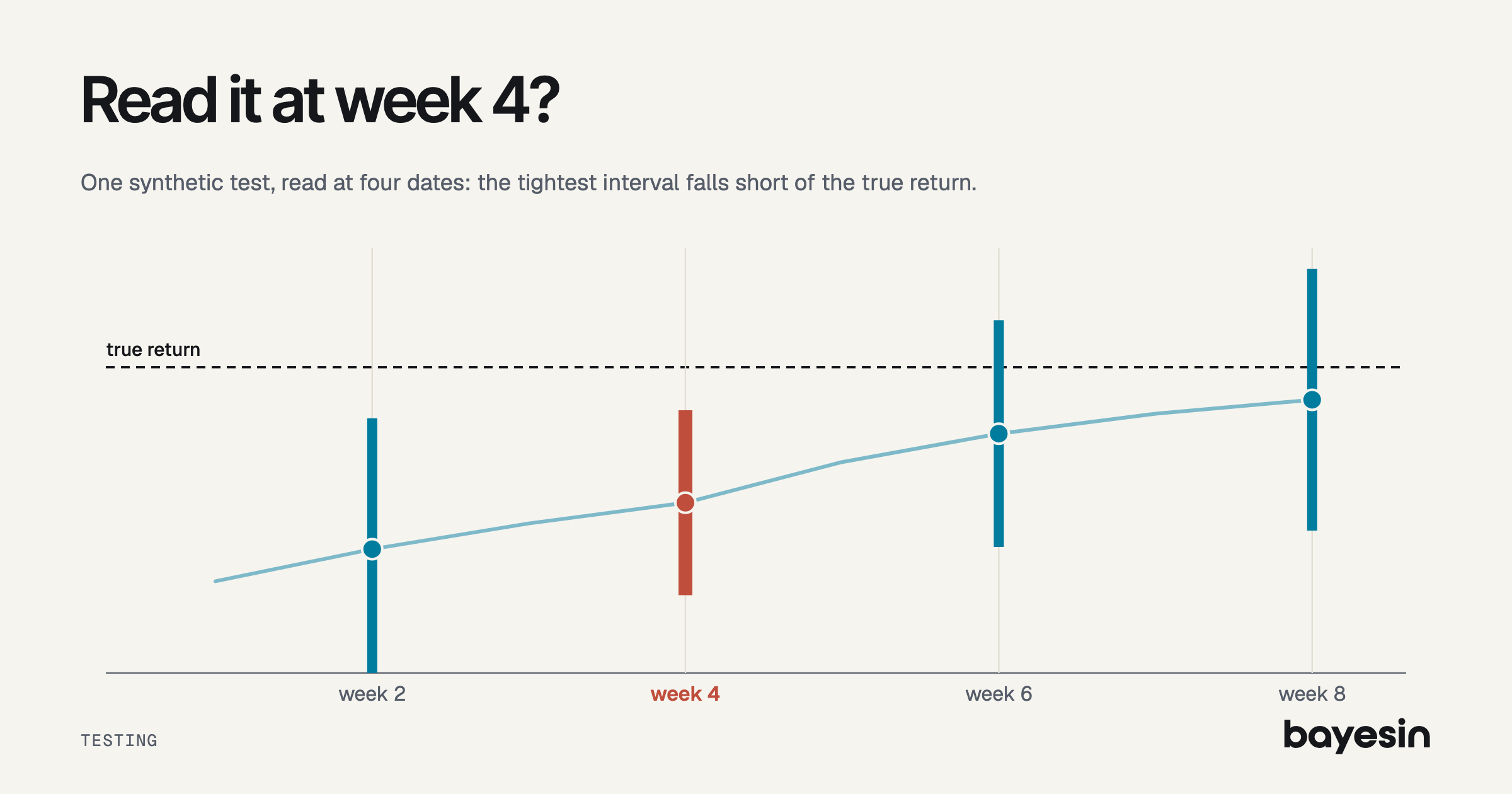
How long to run a test: one synthetic pause read at weeks 2, 4, 6 and 8 shows an early read understating the effect, and a late one only adding noise to it.
Brandon Cade · Nov 9, 2026 · 12 min read
Key Takeaways
- A test runs for its live weeks plus a cooldown.
- In one synthetic pause, week 4 captures 56% of the effect with the tightest interval, which misses the true return.
- Week 8 captures 89%.
- Two half-lives of cooldown is a sound planning default here, though the best week moves with noise.
At the moment a four-week pause ends, this synthetic estimate is 1.00 against a true 1.80, with the narrowest interval the test will ever show. A calendar and a finance review both push you toward that read, and it's short of the truth by nearly half.
Knowing how long to run an incrementality test comes down to seeing what each read date gives you. This post reads one test at four dates, so you can watch the estimate and its interval move in opposite directions. By the end, you'll be able to set live weeks and a read date from your own carryover.
The test here is synthetic, with a known true effect. Its numbers are illustrative, not real customer data. Centers are noise-free, and intervals use independent weekly error.
How long should a test run?
Run the test for the longest of three lengths: one full purchase cycle, the weeks your size needs, and live weeks plus a cooldown. The cooldown should let most of the carryover finish.
Each length answers a different question. The purchase cycle comes first, and GeoLift's walkthrough says a test should contain at least one. Size comes from how big a test needs to be, and carryover is the subject of this post. If you're still deciding where to test, start with which channel to test first.
Two terms carry the rest of this post. Live weeks are when spend is changed. The cooldown is the stretch after spend returns, when you keep measuring, and vendors also call it a post-treatment window. In 2017, Kerman, Wang and Vaver described geo experiments in the same three parts: pretest, intervention and cooldown. For the mechanics of the holdout itself, see how tests are run.
Why does an early read understate the effect?
Because the holdout regions are still running on ads from before the pause, and ads from the test keep working after it ends. The gap opens slowly and closes slowly.
Advertising usually has lag effects, as Jin and colleagues at Google noted in 2017, and I explain what carryover is elsewhere. Here I use geometric carryover with a retention rate of 0.7, which means 70% of the effect survives each week. PyMC-Marketing's GeometricAdstock page links retention and half-life, so a retention of 0.7 gives a half-life of ln(0.5) / ln(0.7) = 1.94 weeks.
The setup is one synthetic brand. Weekly revenue is $510,000, the channel spends $36,000 a week, and its true incremental return is 1.8, set here and unknown in real life. The holdout regions hold 20% of revenue, or $102,000 a week, so the pause withholds $7,200 a week.
During a pause of L weeks, the weekly gap in week t is 1 - 0.7^t, as a share of the full weekly effect. After the pause ends, it's 0.7^(t-L) - 0.7^t. Once it has all played out, the total equals the full return on every dollar withheld.
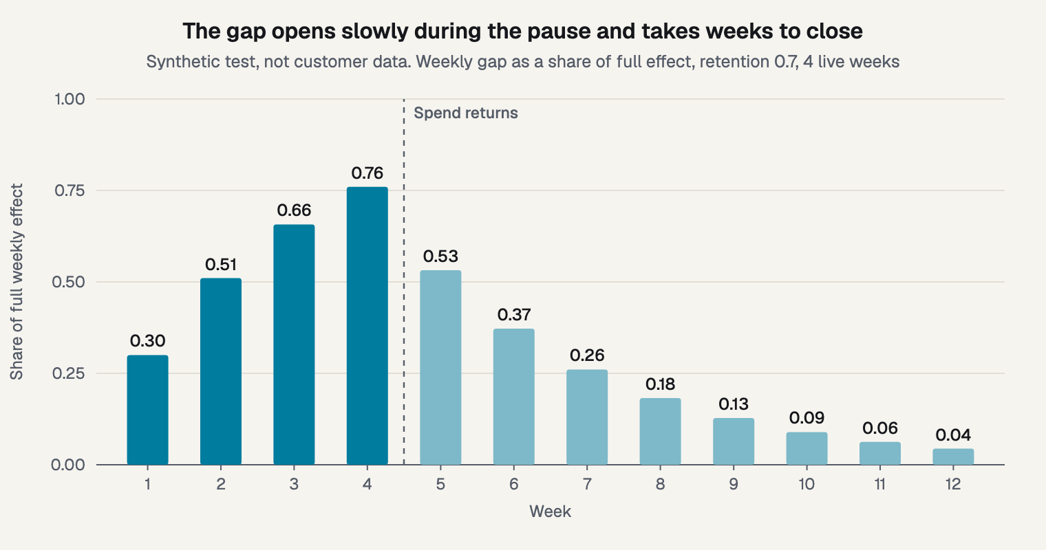
Figure 1. The weekly gap opens over the pause and takes weeks to close.
Add up the bars to get the share captured. Through week 4, the sum is 2.227, so 2.227 / 4 = 55.7% is captured. Through week 8, it's 3.574, so 89.4% is captured. Google's Meridian documentation raises the same concern from the modeling side, warning that short experiments may not capture long-term effects.
One test, read at weeks 2, 4, 6 and 8
The estimate climbs from 0.73 to 1.61 against a true 1.80, while the interval narrows to week 4 and then widens. So the read that looks most certain comes well before the effect has played out.
The pause runs for 4 live weeks, and weekly counterfactual error is 6% of holdout revenue, or $6,120. The expected estimate is 1.8 x captured share. The standard error is $6,120 x sqrt(week) / dollars withheld so far.
- Week 2: Captured: 40.5%; Expected estimate: 0.73; 80% interval: -0.04 to 1.50
- Week 4: Captured: 55.7%; Expected estimate: 1.00; 80% interval: 0.46 to 1.55
- Week 6: Captured: 78.3%; Expected estimate: 1.41; 80% interval: 0.74 to 2.08
- Week 8: Captured: 89.4%; Expected estimate: 1.61; 80% interval: 0.84 to 2.38
Week 4 is the danger. In this synthetic test, the 80% interval at week 4 runs from 0.46 to 1.55, the narrowest of the four. It excludes the true return of 1.80. A real read bounces around that center, yet the interval would contain 1.80 only 27% of the time, against a nominal 80%. That's the lowest coverage of the four reads, ahead of 31% at week 2, 68% at week 6 and 78% at week 8.
The reason is mechanical: by week 4, the most dollars have been changed in the fewest weeks, so noise is smallest relative to dollars. After that, dollars stop accumulating while noise keeps accumulating, and the interval widens as the estimate climbs toward the truth.
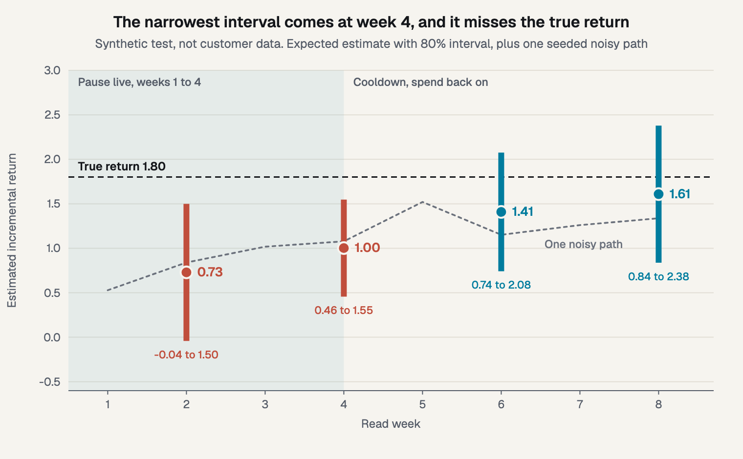
Figure 2. One test at four read dates. Week 4 is the most confident and misses.
The interval here describes noise only: it comes from the test's standard error, so it can't flag a window that ended too early. A credible interval from a model has the same blind spot, because it holds given the model's assumptions, as I cover in reading an interval. Week 2's interval crossing zero isn't evidence of no effect either, because that read is simply early and noisy.
Size belongs in this picture too. Using the 2.8 multiplier from my sizing post, detectable return at week 8 is 2.8 x 0.60 = 1.68. The true return of 1.80 clears that, but the captured estimate of 1.61 doesn't. In other words, compare your detectable effect with the effect the window can capture, not with the full return.
A real read won't look this tidy, and the dotted path on the chart adds one seeded draw of noise to show it. It reads 0.84, 1.08, 1.15 and 1.34 at the four dates, and it hits 1.52 at week 5 before dropping back.
Why not just wait longer?
Because each extra week adds noise, and once the tail has faded it adds little signal. Total error falls, reaches a low point and then rises again.
I combined the two parts as root mean squared error of return: shortfall against the true value, plus noise. Here's what that gives for 4 live weeks at three retention rates, with the lowest value in each column in bold:
- 4: Retention 0.5: 0.60; Retention 0.7: 0.90; Retention 0.85: 1.29
- 5: Retention 0.5: 0.52; Retention 0.7: 0.73; Retention 0.85: 1.14
- 6: Retention 0.5: 0.53; Retention 0.7: 0.65; Retention 0.85: 1.02
- 7: Retention 0.5: 0.56; Retention 0.7: 0.63; Retention 0.85: 0.94
- 8: Retention 0.5: 0.60; Retention 0.7: 0.63; Retention 0.85: 0.88
- 10: Retention 0.5: 0.67; Retention 0.7: 0.68; Retention 0.85: 0.81
- 11: Retention 0.5: 0.70; Retention 0.7: 0.71; Retention 0.85: 0.81
- 12: Retention 0.5: 0.74; Retention 0.7: 0.74; Retention 0.85: 0.81
So the lowest error came 1.0, 1.5 and 1.6 half-lives into the cooldown. The bottom of each curve is flat, which matters more than the exact week. At retention 0.7, for example, week 8 is only 0.9% worse than week 7.
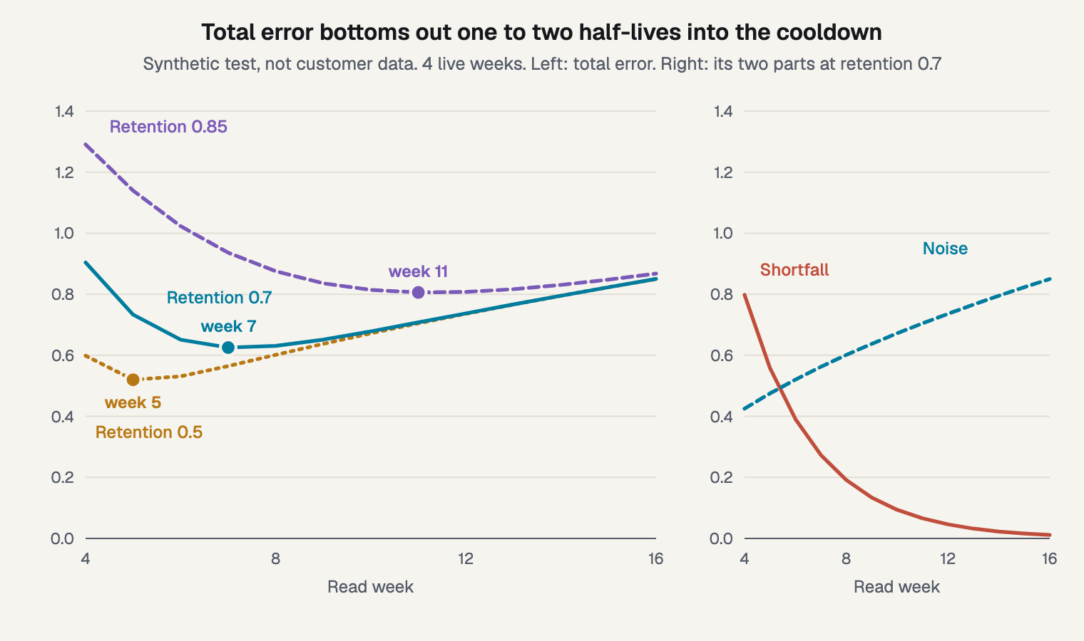
Figure 3. Shortfall falls and noise rises, so total error has a low point.
That low point isn't a law, because it moves with noise and with the return itself. At 3% weekly noise, the best read came 2.0 to 2.8 half-lives in, while at 10% it came about one half-life in. Across 15 scenarios mixing retention, noise, autocorrelation and a lower true return, it ranged from zero to 2.8 half-lives.
Two half-lives is the round number I'd plan with. In those 15 scenarios, a read at two half-lives captured 84% to 94% of the effect. Its total error was at most about 12% above the best week, and at most 2.2% at the base noise. Treat it as a default for this setup, and rerun it on your own noise.
This setup assumes independent weeks, which flatters later reads, because real counterfactuals drift. With autocorrelation of 0.4, the best read at retention 0.7 moved from week 7 to week 6. That's consistent with the noise inflation in my sizing post.
Others make the same point in words. Kerman and colleagues say that if cumulative effects have stopped, more cooldown only adds uncertainty. Robyn's analyst guide notes that longer studies capture long-tail conversions and can add noise. Sellforte, as a vendor, says the same of extra days, and it suggests 30 days after treatment as a starting point.
Brodersen and colleagues showed in 2015 that a model predicting the counterfactual can track impact over time, which is how you'd watch the curve flatten. Decide the rule in advance, though, and don't choose the window by looking for the highest number.
Should you add live weeks or cooldown weeks?
Live weeks buy precision and cost money, while cooldown weeks buy capture and cost calendar time. They fix different problems, so the choice depends on which one you have.
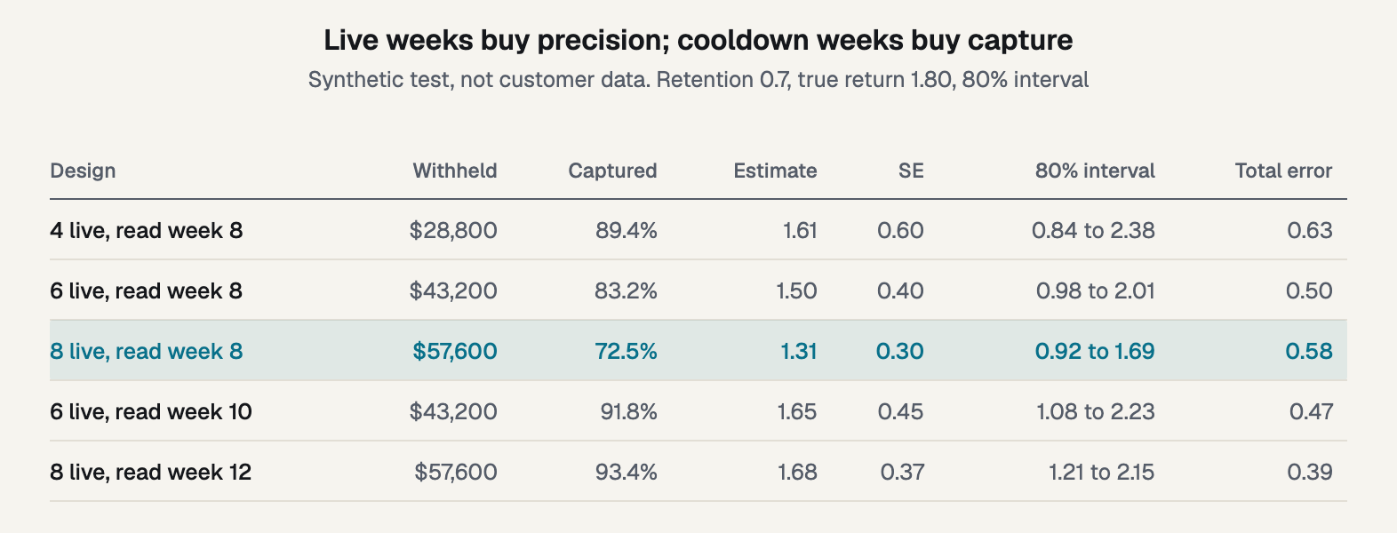
Figure 4. Five designs compared on capture, interval and total error.
Moving from 4 live weeks read at week 8 to 6 live weeks read at week 10 raises dollars withheld from $28,800 to $43,200. Total error falls from 0.63 to 0.47, and the detectable return falls from 1.68 to 1.26. In this setup, that extra $14,400 buys a better test.
Now look at 8 live weeks with no cooldown. It has the tightest interval in the table, 0.92 to 1.69, and it still excludes the true 1.80. Its total error of 0.58 beats the 4 plus 4 design all the same. Total error alone can hide a biased read, so show both numbers.
You can also correct for missed carryover by scaling the estimate with a model's retention. Meridian's tool does this, and it inflates uncertainty as it does, because the correction imports an assumption. There's also one risk I can't size: returning spend may behave differently from before, for example if campaigns have to relearn. Check for it in the cooldown data.
Can you stop early if it looks done?
Look, but don't stop on what you see. Stop early only for harm, a broken test or a data outage.
Looking is fine, and stopping on a threshold is the problem. I ran 2,000,000 no-effect paths with independent weeks, using seed 20261109. Each path checked a threshold at weeks 2, 4, 6 and 8 and stopped at the first crossing:
- 95% interval: Crossing at week 8 only: 5.0%; Crossing at any of the four reads: 12.6%
- 80% interval: Crossing at week 8 only: 20.0%; Crossing at any of the four reads: 42.3%
Half of those crossings are positive, so a team checking an 80% interval at four dates sees a false positive about one time in five. In 2015, Johari, Pekelis and Walsh showed that standard inference is unreliable when you choose sample size by continuous monitoring. They wrote about A/B tests, but the point carries over.
Stopping on a promising read also picks up upward noise, which overstates the effect. Therefore, set the read date in advance and write it down before the test starts. Sequential methods exist if you need a safe way to stop, though they're outside this post.
How do you set the length for your channel?
Get a retention rate, convert it to a half-life, then set the read date at live weeks plus about two half-lives. Check that against your calendar.
- Get a retention rate. Take it from your model, with its interval, or from the channel's buying cycle if you have no model.
- Convert it. Half-life = ln(0.5) / ln(retention). A retention of 0.85 gives 4.27 weeks, and 0.5 gives 1.
- Set live weeks from size. Use the detectable effect, against the share you'll capture.
- Add the cooldown. Two half-lives is a starting point. Lean shorter when your noise is high.
- Count backward from blackout dates. A test starting this week would run into Black Friday on 27 November, so plan for January.
Published ranges are a useful check, as long as you read them as vendor data. Haus, a direct competitor, reports that Meta experiments on its platform average 18.6 active days plus 8.8 cooldown days. It recommends 3 to 4 active weeks plus 2 weeks of cooldown for YouTube.
Stella's benchmarks cover 225 geo tests, with a median of 33 treatment days. Of those, 55.6% included a post-treatment window, with a median of 8 days. Stella's users are self-selected, and its authors advise discounting the results.
Frequently asked questions
What is a post-treatment window?
It's the same thing as a cooldown: the weeks after the change ends when you keep measuring. Spend is back on, but the gap between holdout and control is still closing. In my synthetic test, the cooldown lifts captured share from 55.7% at week 4 to 89.4% at week 8.
How long should a cooldown be?
Two half-lives is a sound starting point in my setup, though the lowest error ranged from zero to 2.8 half-lives across the scenarios I ran. Check when the cumulative effect stops rising. Noisier data favors a shorter cooldown, and a longer one suits low noise and long carryover.
Is two weeks ever enough?
Yes, for a short buying cycle and little carryover, if the size also works. At a retention of 0.5, the half-life is one week, so two weeks of cooldown is two half-lives. Two weeks in total is harder, because the dollars withheld and the captured share are both small.
Should I run through a holiday?
Avoid it where you can. A holiday changes baseline demand and can change how channels behave, so the comparison between regions gets harder to trust. If your window has to include one, keep the same regions and read date, and treat the result as specific to that period.
What to do before the test starts
Put a read date on your next test before it starts. Three things set it:
- Take the longest of the purchase cycle, your size requirement, and live weeks plus cooldown.
- Fix the read date in writing.
- Don't stop on a good-looking read.
You can see how carryover is modeled in Bayesin: the model estimates carryover per channel, and every figure carries its interval. Your team runs the test, and Bayesin tracks it and reads the result.
Sources
- Google, "Estimating Ad Effectiveness using Geo Experiments in a Time-Based Regression Framework," Kerman, Wang and Vaver, 2017
- Google Meridian, "Calibrate treatment priors," documentation, 2026
- Meta Robyn, "An Analyst's Guide to MMM," documentation, undated
- Meta open source, "GeoLift Walkthrough," documentation, undated
- Google Research, "Bayesian Methods for Media Mix Modeling with Carryover and Shape Effects," Jin et al., 2017
- PyMC-Marketing, "GeometricAdstock," API documentation, undated
- arXiv, "Always Valid Inference: Bringing Sequential Analysis to A/B Testing," Johari, Pekelis and Walsh, 2015
- Annals of Applied Statistics, "Inferring causal impact using Bayesian structural time-series models," Brodersen et al., 2015
- Haus, "How long should you run an incrementality test for?," vendor guide, 2026
- Stella, "2025 DTC Digital Advertising Incrementality Benchmarks," vendor report, 2026
- Sellforte, "How long should we measure sales after an incrementality test ends?," vendor guide, 2026
See it on your own rows.
Bayesin is pre-launch. Join the waitlist and we will reach out as access opens.
Get new posts by email.
New posts only. See privacy for what we keep.