Testing
No regional data? What a national spend pulse can tell you
A national spend pulse has no control group, so its limits matter. See how big it must be, what a demand shift does to it, and when to choose another test.
Brandon Cade · Nov 19, 2026 · 12 min read
Key Takeaways
- A national spend pulse compares results with a forecast, so it's the weakest test design.
- In my synthetic map, only a full shutdown at a 1.5 return reached "enough" without a reference series.
- A 3.5% demand shift takes every cell with an effect below "enough," and the interval doesn't widen.
- Check for regional data first.
At this synthetic brand's noise, a 30% national cut is hard to tell from an ordinary week. Across 1,000 simulated runs at a true return of 1.5, the 95% interval caught that cut 21% of the time.
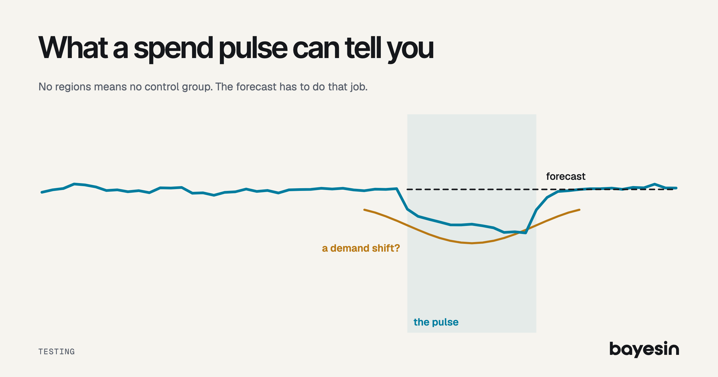
A geo test compares regions with each other. With no regions, you have no control group, so a forecast has to do that job. A national spend pulse is a planned change in a channel's national spend, read against that forecast.
This post shows how to size a pulse, how to run one, and how to see when it isn't enough. Every number here is synthetic: illustrative, and not customer data.
Do you really have no regional data?
Check this first, because a geo test is the stronger design and you may already have what it needs. You need two things: an outcome by region, and a way to change spend by region.
Order data with a shipping location often gives you the first, even when no report shows it. Most ad platforms can target by region, which gives you the second. Google's Meridian documentation makes a related point for models: too little variation in spend hurts national models. It also suggests geo granularity when a national model is short of data.
Regions needn't be many, either. In 2017, Kerman, Wang and Vaver at Google showed that time-based regression can predict a counterfactual from few regions. It still needs a control region.
A pulse is the real option when the media only buys nationally, when you have too few regions, or when no regional outcome exists. If you're still choosing what to test, pick the channel first. And if the channel has run flat for years, a pulse also gives a model the variation it needs.
What can a pulse tell you, and what can't it?
A pulse measures the gap between actual results and a forecast, so the forecast does the work of a control group. That gap can show a large change moved revenue in that window. It can't rule out everything else that changed.
The design has a name in other fields: an interrupted time series. In 2017, Bernal, Cummins and Gasparrini called it "one of the strongest evaluative designs when randomization is not possible" in public health. They also say it's exposed to confounders that move quickly, and that it works best on short-term outcomes. The method transfers to media.
Google's CausalImpact documentation states two assumptions for this kind of read. Any control series must be unaffected by the intervention, and its relationship with your outcome must stay stable through the test. If a control was affected, the page warns, you can misestimate the effect or conclude there was one when there wasn't. The method comes from Brodersen and colleagues, in 2015.
Gordon, Moakler and Zettelmeyer compared two observational methods with 663 Facebook experiments. The better method's median absolute gap in lift was 115, 107 and 62 percentage points for the upper, middle and lower funnel. Median experimental lift was 28%, 19% and 6%. Those are user-level methods rather than pulses, so read them only as a warning about reads without a control group.
How big does the pulse have to be?
At $740,000 of weekly revenue and this noise, only a cut of 60% or more can clear the bar by hand. A simulated read sets the bar higher still.
Here's the setup. The channel spends $58,000 a week. Weekly residual noise around the forecast is 3.5% of revenue, or $25,900. The test runs 6 live weeks, with autocorrelation of 0.5. That last input matters, since Bernal and colleagues note that consecutive observations tend to resemble each other. Here's the arithmetic, using the 2.8 multiplier from the MDE, by hand:
- Standard error if weeks were independent: Calculation: 25,900 / sqrt(6); Result: $10,574
- MDE if weeks were independent: Calculation: 10,574 x 2.8; Result: $29,606 a week
- Variance inflation at autocorrelation 0.5: Calculation: 1 + 2 x (5/6 x 0.5 + 4/6 x 0.25 + 3/6 x 0.125 + 2/6 x 0.0625 + 1/6 x 0.03125); Result: 2.34375
- Standard error with autocorrelation: Calculation: 25,900 x sqrt(2.34375 / 6); Result: $16,187.50
- MDE with autocorrelation: Calculation: 16,187.50 x 2.8; Result: $45,325 a week
The MDE is what the test can detect at a two-sided 95% threshold and 80% power. It's a frequentist planning figure, and the read can still report a credible interval. The expected effect is what the channel might do, which is spend change times true return:
- Cut 30%: Spend change a week: $17,400; True return 0.8: $13,920: below; True return 1.5: $26,100: below
- Cut 60%: Spend change a week: $34,800; True return 0.8: $27,840: below; True return 1.5: $52,200: above
- Off (100%): Spend change a week: $58,000; True return 0.8: $46,400: above; True return 1.5: $87,000: above
Autocorrelation raises the MDE 1.53 times, from $29,606 to $45,325. It moves no cell in this table, but it removes the margin. A shutdown at a return of 0.8 now clears by $1,075, or about 2%. An 80% interval as the threshold gives a multiplier of 2.12 and a bar of $34,318, and the table still doesn't change. It would let 1 in 10 no-effect tests show positive lift from noise. With no control group to catch that, I'd keep the 95% threshold.
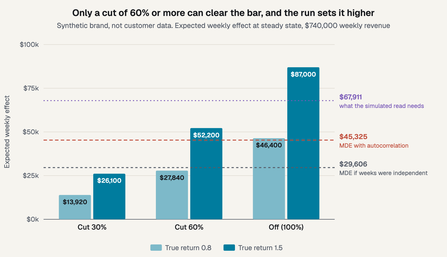
Figure 1. Expected effect against the hand MDE and the simulated bar.
Treat that hand MDE as a floor, because the simulation below shows why. Its 8-week read has a median standard deviation of $139,554, against $97,125 for the hand figure's 6-week total. That's 1.44 times the noise, since a real read also carries forecast error and two extra weeks.
Carryover takes a share too. With a decay of 0.5, the read captures 5.75 weeks' worth of steady-state effect. So 2.8 x $139,554 / 5.754 gives a bar of $67,911 a week. A shutdown at 0.8 falls below that, and it was detected in only 47% of runs. Even large randomized tests struggle here: Lewis and Rao found a median interval on return over 100 percentage points wide across 25 experiments.
Why can't the interval warn you about a shock?
A credible interval describes uncertainty given the model, and a shift the model doesn't know about moves the estimate without widening the interval. So the failure doesn't show on the page.
A 3.5% shift in demand is $25,900 a week, almost the same as the 30% cut's $26,100 at a return of 1.5. Over 8 weeks, that's $207,200 of revenue the forecast knows nothing about.
The width of the 80% interval had a median of $360,145 in the calm calendar and in both shifted ones. The two can't differ, because the forecast is built from weeks before the test. Mean error, meanwhile, went from $1,829 to $209,029 with demand up, and to -$205,371 with demand down. The 80% interval held the truth 78% of the time in a calm calendar, and 43% and 41% under a shift.
A credible interval is the range where the effect probably sits, given the model and data. I go through what an interval does and doesn't say elsewhere. It isn't a check that the model is right, and that's the gap a shock falls through.
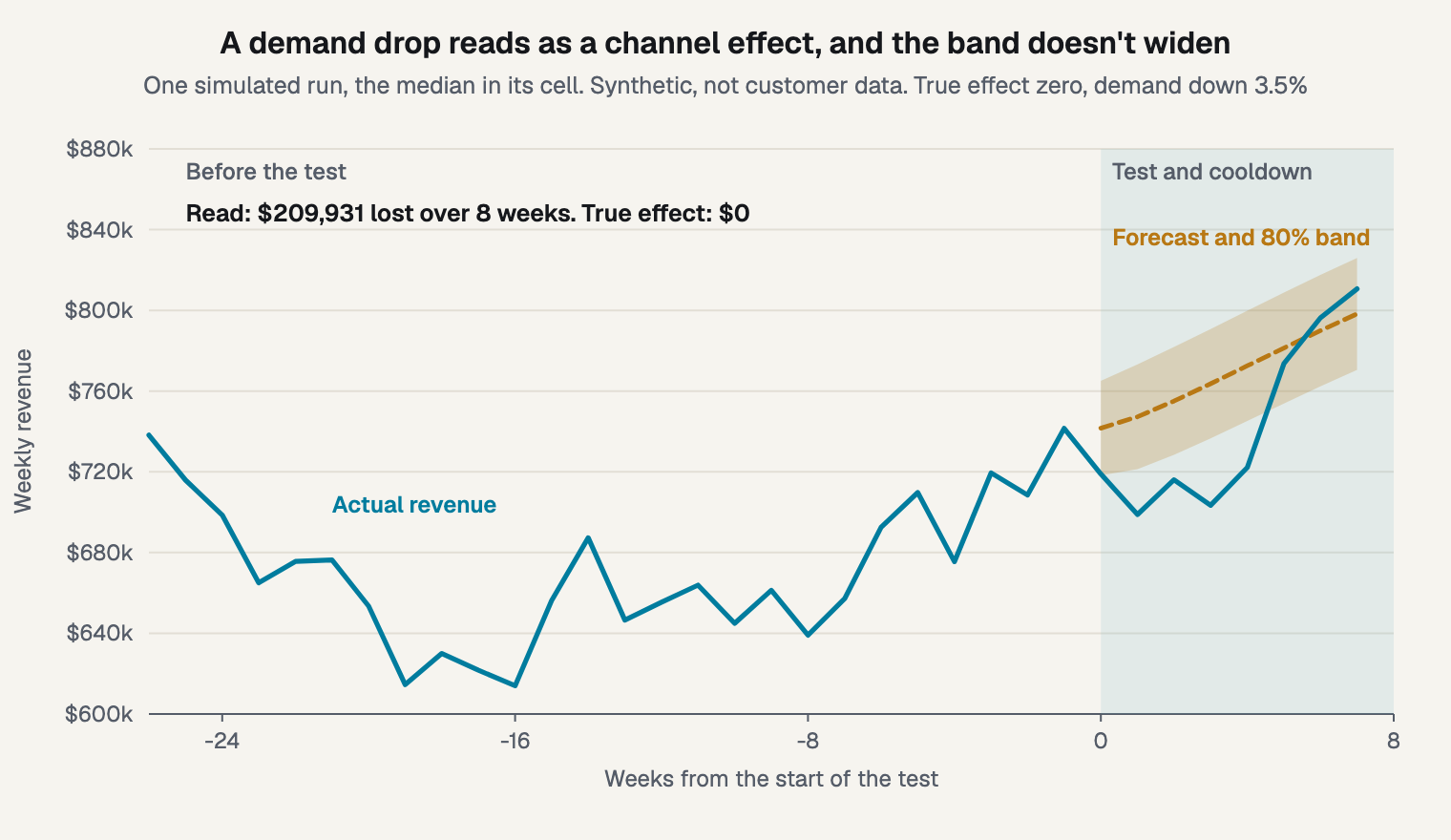
Figure 2. One simulated run, the median in its cell: a channel with no effect, in a demand drop.
That run reports $209,931 lost, with an 80% interval of $79,321 to $340,540 lost. Its 95% interval also excludes zero, if only just, and the true effect is zero. It's the run closest to the median, so it isn't an extreme case. Across all runs, a channel with no effect showed a result 32% of the time under a shift, against 5% in a calm calendar.
When is a pulse enough, and when isn't it?
It's enough when the change is large, the calendar is clean, something unaffected tracks your demand, and the decision can be reversed. The map below shows how few cells get there.
I simulated 104 weeks of history, 6 live weeks and 2 cooldown weeks, with 1,000 runs per cell and seed 1907. Revenue has a 5% annual trend and 12% seasonality, and noise is 80% shared demand and 20% specific to the series. The read is a Bayesian linear regression with weak priors, trend, seasonal terms and autocorrelated errors, fit on the weeks before the test.
The reference series is a second revenue line that shares the demand factor and any shock, and the pulse can't touch it. An unadvertised product line or a market the channel doesn't reach might qualify. The simulation grants that assumption, and in real use that's the whole problem.
I ran the calibration first, on zero-effect, calm-calendar cells. False alarms at the 95% threshold were 5.2% with no reference and 6.9% with one, against a nominal 5%. The 80% interval held the truth 78.0% and 76.8% of the time, so it runs slightly narrow.
The verdict rule was set before the run. Enough means 80% detection, 80% interval coverage within 5 points of nominal, and mean error under 25% of the true effect. Directional passes the error and coverage tests with 50% to 80% detection. Under no effect, a cell is a false result if more than 10% of runs exclude zero.
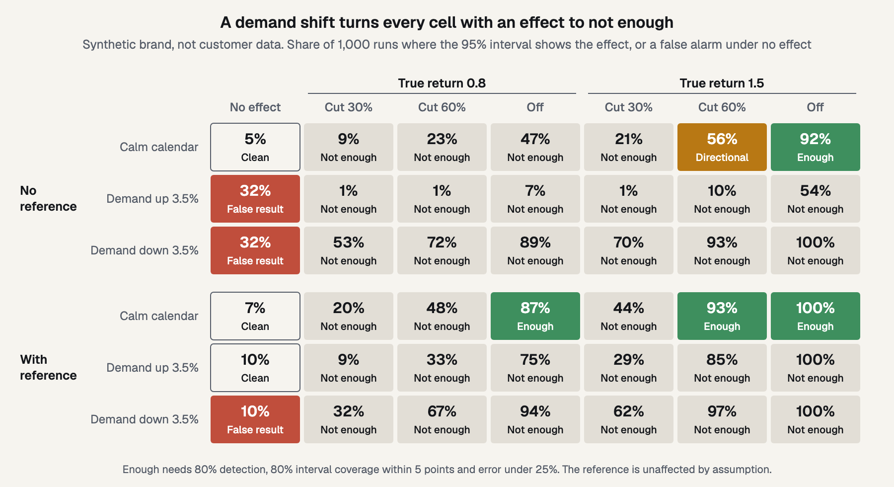
Figure 3. Detection share and verdict for each simulated cell. Four things stand out:
- With no reference, one cell passes. A shutdown at a return of 1.5 reached 92% detection. A 60% cut at 1.5 reached 56%, which is directional.
- A shift defeats everything. Detection can look superb. A shutdown at 1.5 hit nearly 100% with demand down, while its mean error was 41% of the true effect.
- A reference series helps a lot. It cut the read's standard deviation by 41%, to $82,758, and the bar to $40,272. Mean error under a shift fell from about $207,000 to $37,016 and $44,109.
- It doesn't fully rescue a shifted calendar. Coverage fell to 74% and 72%, below the 75% floor. Those cells failed even at 100% detection and error under 10%. False alarms sat at about 10%, either side of my line, so read those two as one result.
A smaller channel fares worst. At $15,000 of weekly spend with no reference series, the best cell, a shutdown at a return of 1.5, reached 17% detection.
The table below is my judgment, supported by the map where it has a cell. The long sales cycle row rests on Bernal and colleagues. Prose Media, an agency, also calls the time-based pulse the weakest of its three designs. It's useful for stopping wasteful spend, not for large annual reallocations.
- Large change, clean calendar, unaffected reference series, reversible decision: Enough to act on, with the interval stated
- Large change, clean calendar, no reference series: Directional at best: enough to stop clearly wasteful spend, not to set next year's budget
- Change smaller than the MDE: Not enough. Change the size or don't run it
- Promotion, launch, price change or peak in the window: Not enough
- Long sales cycle or long carryover: Not enough
- Channel is a small share of spend: Not enough
- A large or hard-to-reverse budget decision: Not enough. Find regions or use a platform lift study
How to run one
Write the model and the read date down before spend moves. Bernal and colleagues recommend specifying the impact model in advance, so you don't find effects in random fluctuation. Then take these steps:
- Write it down. Record the expected effect, the read date and the threshold.
- Pick a clean window. Avoid promotions, launches and price changes, and see why a peak makes a poor window.
- Hold everything else steady. That covers other channels and prices, since a pulse can't separate two changes.
- Choose a reference series the pulse can't touch. If your ads could move it, it isn't one.
- Make the change large and hold it. Decide whether to cut or add first. Your team makes the change in the ad platforms.
- Read it with an estimator separate from any model it may inform. It's a common rule against circular reasoning.
Then let the carryover finish before you read.
Repeating the pulse may help. Bojinov, Simchi-Levi and Zhao and Hu and Wager study repeated on-off designs under carryover. Hu and Wager show that dropping the periods right after each switch reduces bias. That work uses short periods, so it's only an analogy for weekly media.
Frequently asked questions
Is a pulse the same as a before-and-after comparison?
It's a before-and-after comparison with a forecast, which beats a raw one because it accounts for trend and season. It shares the main weakness, though. Anything else that changes during the window lands in the estimate, and in my simulation a 3.5% demand shift produced about $207,000 of error.
Can I use branded search as a reference series?
Only if your ads can't move it, and they usually can. Advertising often lifts branded searches, so the reference would rise and fall with your own pulse and hide part of the effect. An unadvertised product line or a market the channel can't reach is a safer place to look.
Should I cut or add?
A cut saves spend and usually gives a bigger signal, since a response curve is steeper below today's spend. An increase answers a different question, which is what the next block earns. Pick the direction by your budget decision, then size the change against your MDE before anything moves.
How long should a pulse run?
Long enough for carryover to finish, plus the weeks your MDE needs. Longer live periods help the arithmetic, but each added week gives demand another chance to shift. In my simulation, 6 live weeks and 2 cooldown weeks captured 5.75 weeks' worth of steady-state effect, at a decay of 0.5.
Can I feed the result into my model?
Yes, with its full uncertainty, and with the calendar conditions noted beside it. Don't read the test with the same model it will update, because that's circular. If demand may have shifted in the window, say so and widen the uncertainty, since the interval won't do that by itself.
Check for regions first
If you truly have no regional outcomes, run the sizing table on your own revenue, noise and spend, then check the verdict table.
Sources
- International Journal of Epidemiology, "Interrupted time series regression for the evaluation of public health interventions: a tutorial," Bernal, Cummins and Gasparrini, 2017
- Google open source, "CausalImpact," package documentation
- Annals of Applied Statistics, "Inferring causal impact using Bayesian structural time-series models," Brodersen et al., 2015
- Marketing Science Institute, "Close Enough? A Large-Scale Exploration of Non-Experimental Approaches to Advertising Measurement," working paper 22-106, 2022
- Quarterly Journal of Economics, "The Unfavorable Economics of Measuring the Returns to Advertising," Lewis and Rao, 2015
- Google for Developers, "Amount of data needed," Meridian documentation
- Google Research, "Estimating Ad Effectiveness using Geo Experiments in a Time-Based Regression Framework," Kerman, Wang and Vaver, 2017
- arXiv, "Design and Analysis of Switchback Experiments," Bojinov, Simchi-Levi and Zhao, 2020
- arXiv, "Switchback Experiments under Geometric Mixing," Hu and Wager, 2022
- Prose Media, "Incrementality testing: 3 tests you can run this month," agency opinion, 2026
See it on your own rows.
Bayesin is pre-launch. Join the waitlist and we will reach out as access opens.
Get new posts by email.
New posts only. See privacy for what we keep.