Planning and forecasting
Reading your holiday weeks: what one peak can teach a model
One holiday peak can size your pull-forward and test a forecast, but it can't split media from discounts. Freeze your forecast now, then read net lift.
Brandon Cade · Nov 12, 2026 · 11 min read
Key Takeaways
- One peak can size your pull-forward and test a forecast you froze beforehand.
- It can't split media from discounts and demand, because all three move together.
- Write down your forecast and promotions before 27 November.
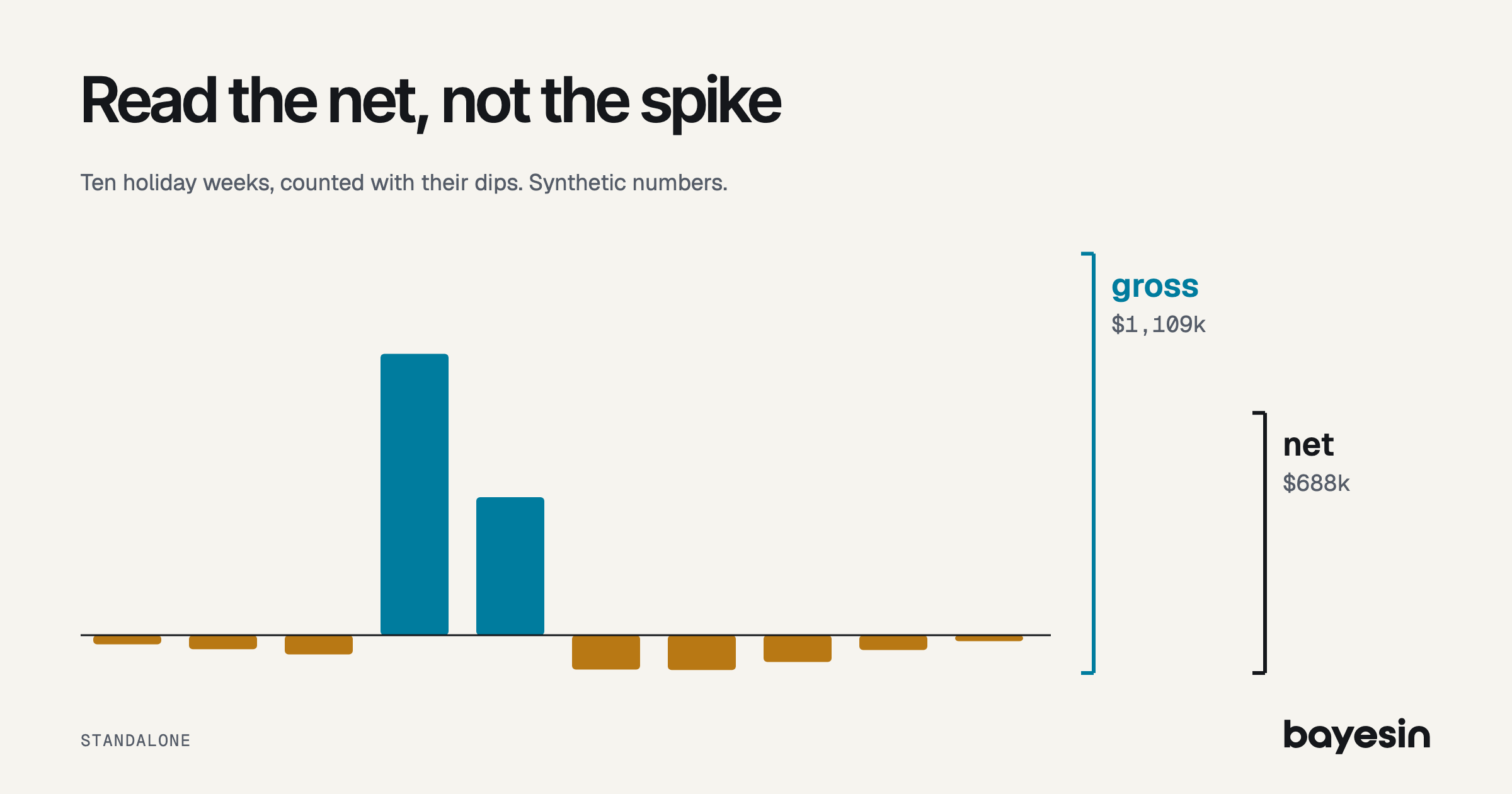
- In a synthetic ledger, a $1,109k spike nets to $688k, or 62% of it.
Adobe counted $44.2 billion in US online spending over the five days from Thanksgiving to Cyber Monday 2025. Your own peak is probably your biggest stretch of the year too, so it gets read harder than any other.
The trouble with BFCM marketing measurement is that spend, discounts and demand all rise in the same few days. The spike looks like proof of something, and it's hard to say of what. This post gives you three things to write down before 27 November and one calculation to run in January. It also shows, with a small simulation, what a model can and can't learn from those weeks. I built every number from the ledger onward for this post, so they're synthetic, and none of it is customer data.
What can one holiday peak teach a media mix model?
One peak teaches two things well: how much of the spike was new revenue, and whether your forecast held. It teaches little about media, because media isn't the only thing moving.
Google researchers Chan and Perry described the underlying problem in their 2017 review. When media is targeted toward seasonal demand, the two rise together, and that creates selection bias. Proxies for demand may not fully capture it. I've written separately about how the calendar enters a model, so here I'll stick to what you can do after a peak.
A peak can:
- Size your pull-forward, by counting the dips on either side of the spike.
- Check a forecast, if you froze one before the weeks arrived.
A peak can't:
- Separate media from discounts and demand.
- Give you a marginal return that holds in January, when demand and spend are both different.
- Settle a change from last year, because one comparison is a lead rather than a measurement.
Before 27 November: what should you write down?
Three items take little time now and can't be rebuilt later: a frozen forecast, a promotion log and a spend log. People's memories of why a Tuesday looked odd won't last until January.
- A frozen forecast. Save your forecast of each week, with its interval, by 26 November at the latest. Before the peak week begins on 23 November is better, since those days then can't inform it.
- A promotion log. Record discount depth, sitewide or category, start and end dates, stockouts and shipping cut-offs.
- A spend log. Keep spend by day and by channel, even if your model reads weeks.
Black Friday falls on 27 November this year, so there's still time. Google Meridian's control variables page suggests asking marketing managers whether spikes in spend correspond to events such as holidays. Ask that this month and write down the answer while people remember it.
One thing not to start now is a test. Sellforte, a vendor, warns that a test during peak trading "may answer a seasonal question" rather than give a useful annual baseline. It also flags the risk of lost margin. Use the quiet weeks ahead to decide which channel to test first instead.
How do you read net lift instead of the spike?
Add the dips to the spike. In this synthetic ledger, $1,109k of gross lift nets to $688k, because $421k of it came out of the weeks around the peak.
You need one extra column: expected revenue, meaning what you'd have booked with no promotion and no extra media. In practice, it comes from prior years or a model fit, and it carries its own uncertainty. It isn't the forecast you froze, because that forecast includes your planned promotion and media.
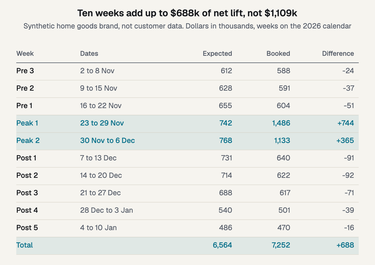
Figure 1. The peak ledger, for a home goods brand that doesn't exist. Rebuild it with your own weeks.
The arithmetic is short:
- Gross peak lift: 744 + 365 = $1,109k.
- Dip before the peak: 24 + 37 + 51 = $112k.
- Dip after the peak: 91 + 92 + 71 + 39 + 16 = $309k.
- Net lift: 1,109 - 112 - 309 = $688k, or 62% of the gross figure.
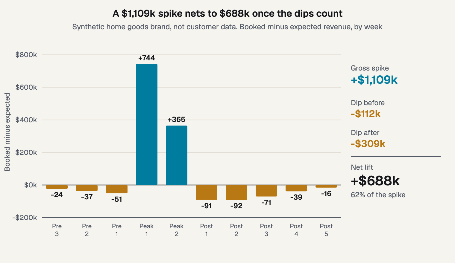
Figure 2. The same ledger drawn as differences, so the dips are visible.
The added peak media here is $312k, which gives $3.55 of gross lift and $2.21 of net lift per added dollar. The second ratio still isn't a media return. Net lift holds the discount, the season's demand and the media together. The ledger answers "how much of the spike was new revenue?", and it doesn't answer "what did media do?"
The expected column deserves some suspicion. Across these ten weeks it totals $6,564k, so a 1% error in its level moves net lift by $66k. A 2% error either way gives a range of $557k to $819k, which is why I'd report net lift as a range. Your own window should also run long enough to catch the dips. This one ends on 10 January, so you can't finish it in the first week of the year.
The dips here are assumptions of the example. Some brands will show little or no dip. Public evidence on size is thin: Monks, an agency, reports a "brought forward" effect from its own modeling work and gives no size. So treat that as directional, and let your ledger decide.
Did your forecast hold?
Compare the booked weeks with the interval you froze. An 80% interval misses about one week in five by design, so one miss isn't a verdict on the model.
The live post on what a forecast interval tells you covers how to read that width. Peak weeks add one complication, because they aren't independent of each other. The same discount and the same demand run through both, so two misses in a row aren't two separate pieces of evidence.
When a miss is large, open the logs before you touch the model. A deeper discount, a stockout or an early shipping cut-off is a more likely reason, and you can check it in minutes. That's the payoff for writing them down this month.
If nothing explains the miss, it's a useful finding in itself. Keep it for the next fit and note it in your plan, rather than reading it as a verdict on media.
Why can't one peak separate media from discounts and demand?
A term for the peak week absorbs that week, and leaving the term out hands the spike to media. Neither path teaches much about media, and a simulation shows the size of each.
Forecasting: Principles and Practice describes a spike variable as equivalent to a dummy for handling an outlier, one that removes the week's effect. A week with its own term gets fitted exactly, so it adds nothing to the media estimate. Leave the term out, and the media estimate absorbs much of the spike.
To size this, I simulated 500 synthetic brands over 104 weeks. Each has one channel, a true return of 1.30 and no carryover, so the mechanics stay visible. Baseline is $600k a week, with 15% yearly seasonality and noise of 5% of baseline. Media averages $60k a week and rises to 2 to 3 times normal in two peak weeks a year. Holiday demand adds 60% of baseline in those weeks, moving up to 15% either way by year.
I fit each brand three ways, with a Normal(1, 1) prior on the return. Each fit has two yearly Fourier pairs, the form PyMC-Marketing's example sets with yearly_seasonality=2. An 80% credible interval here holds the true return with 80% probability, given the model and prior. It says nothing about whether the model is the right one, and model A below shows why that matters.
- A: no holiday term: Mean estimate: 3.12; Interval width: 0.61; Intervals holding 1.30: 0%
- B: one term per peak week: Mean estimate: 1.28; Interval width: 0.52; Intervals holding 1.30: 81%
- C: one shared term: Mean estimate: 1.28; Interval width: 0.47; Intervals holding 1.30: 78%
- C, bigger years get more spend: Mean estimate: 1.32; Interval width: 0.48; Intervals holding 1.30: 77%
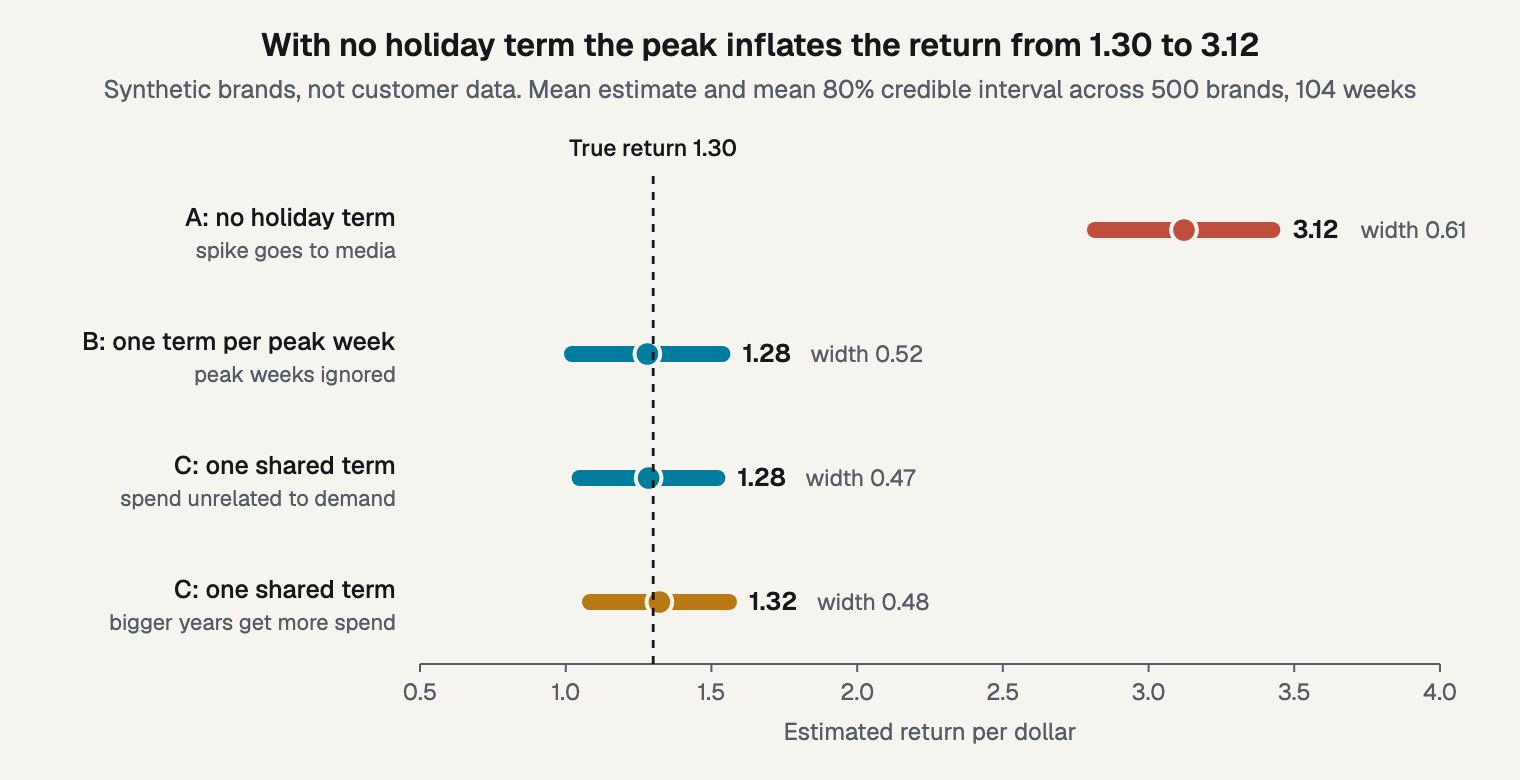
Figure 3. Leaving the term out more than doubles the return, and its interval never holds the truth.
Model A is the warning: it reports 3.12 against a true 1.30, and its interval held the truth in none of the 500 brands. That interval is only slightly wider than the others, so width alone won't warn you.
Model B recovers the return from the ordinary weeks and ignores the peaks. Model C does let peak weeks speak, and its interval is 8.5% narrower than B's. Its estimates are no closer, though: the root mean square error is 0.194 in both. So the peak weeks made the interval look better without making the estimate better.
I expected a clear bias in C when peak demand varies by year, and I found none in this run. It stays at 1.28, a shade below truth, which is the direction a prior centered on 1 pulls. When I made bigger years get more spend, C moved only to 1.32. That's small here, and these brands have no carryover or discount term, so don't read it as a general rule.
The same logic holds on a hand calculation. Say last year added $260k of peak spend for $980k of peak lift, and this year added $312k for $1,109k. The slope is 129 / 52 = 2.48. Now assume weekly unexplained noise of $60k. A two-week lift then has a standard deviation of 60 x sqrt(2) = 84.9, and the difference of two years has 120. The slope's standard error is 120 / 52 = 2.31.
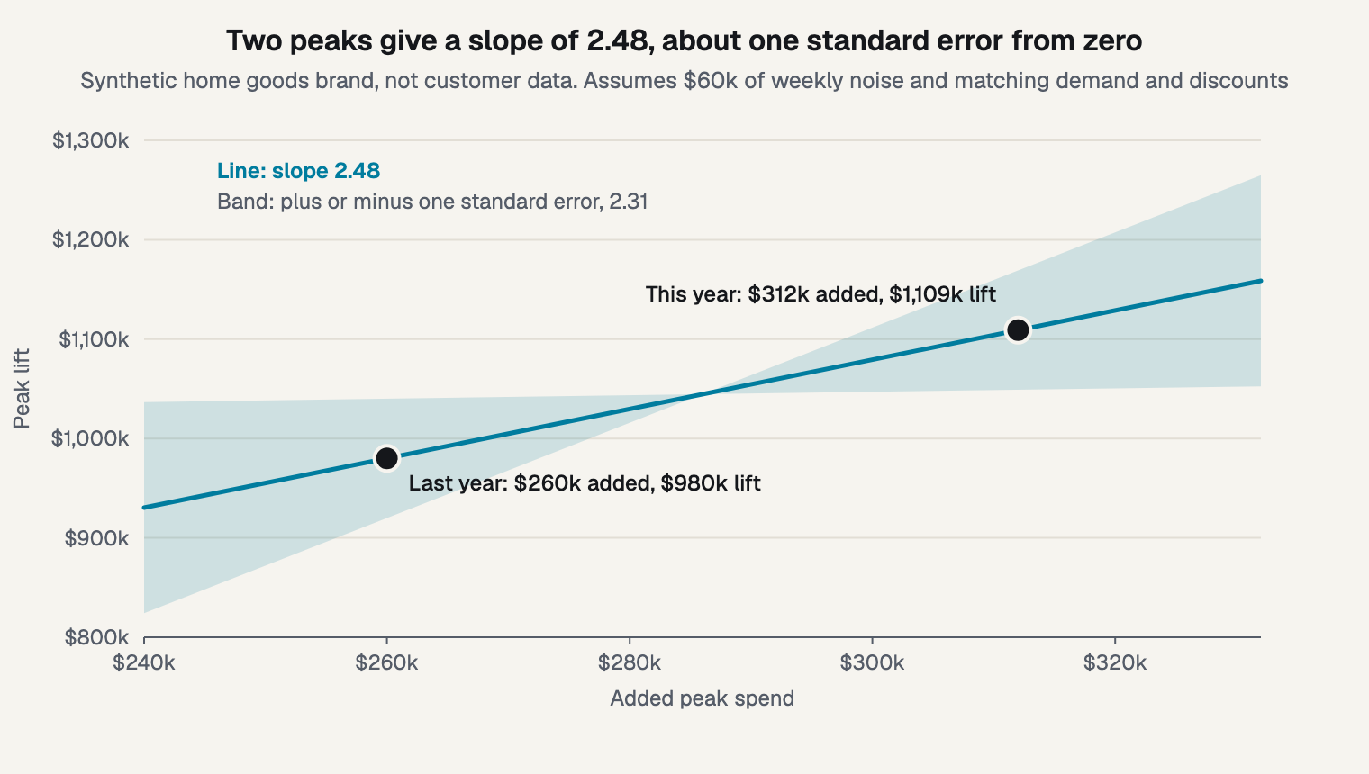
Figure 4. Two synthetic peaks give a slope about one standard error from zero, assuming matching demand and discounts.
An 80% range on that slope runs from -0.48 to 5.44. It also assumes demand and discount depth matched in both years, which is rarely true. One comparison is a lead, not a measurement.
Two more findings point the same way. Chan and Perry note that fitting on a limited range brings high uncertainty when you extrapolate. Peak spend sits outside your normal range, in a different demand state. Jin and colleagues at Google showed in 2017 that priors can strongly affect results when the sample is small.
Tools handle the calendar differently. Robyn's analyst guide aggregates holidays into one variable by default and advises adding your own sales events. Meridian's national default is a single knot, effectively a common intercept, so a national model needs knots set before it can see the calendar. Both docs can change, so check the current pages.
What should change in your plan for next year?
Vary something on purpose. Change peak spend or discount depth by a known amount, and log it, so that next year's comparison means more than this one.
Don't carry a peak marginal return into January. In the simulation, model B got its answer entirely from ordinary weeks, and the peak weeks added almost nothing. That's where the next round of learning is too. A Q1 test can read a channel in normal demand. Start with how big a test needs to be, then let the carryover finish.
Frequently asked questions
Does Black Friday pull sales forward?
Sometimes, and the size varies by brand. Your ledger shows it directly, as dips in the weeks around the peak. Monks, an agency, reports a brought-forward effect from its own modeling and gives no size, so treat that as directional. The dips in my example are assumptions, not findings about any brand.
Should I run a test during the peak?
Usually not, if you want an annual read. Sellforte, a vendor, warns that a peak test may answer a seasonal question, and it flags lost margin too. A test in normal weeks gives you a return you can use across more of the year. Plan one for January instead.
Can I fit a model with only one holiday season?
Yes, with wider intervals. In my simulation, 52 weeks with one term per peak week gave an interval width of 0.74, against 0.52 with 104 weeks. A short history often produces a wide interval rather than no answer, and I cover how many weeks a fit needs separately.
Is the holiday peak part of the baseline?
In many models, yes. Baseline holds the revenue that would have arrived without media, and seasonal demand belongs there. Promotions usually get their own terms. If the peak stays out of the baseline, the media estimate absorbs much of the spike, as model A shows. See how the calendar enters a model.
What to do this week
Freeze your forecast, start the promotion log and turn on daily spend exports this week. Then, once the second week of January arrives, build the ledger and write your net lift as a range.
Bayesin fits your yearly pattern from your own history once it covers a full year, so a holiday peak lands in the baseline. There's more on how Bayesin treats seasonality and promotions on the ecommerce page. If you'd like to see it on your own weeks, you can request access.
Sources
- Adobe, "Adobe: Cyber Monday Hits Record $14.25 Billion in Online Spending with Over $1 Billion Driven by Buy Now Pay Later," press release, 2025
- Google, "Challenges And Opportunities In Media Mix Modeling," Chan and Perry, 2017
- Google Research, "Bayesian Methods for Media Mix Modeling with Carryover and Shape Effects," Jin et al., 2017
- OTexts, "Forecasting: Principles and Practice," chapter 7, "Time series regression models", undated
- Google Meridian, "Control variables," documentation, undated
- Google Meridian, "Model specification," documentation, undated
- Meta Robyn, "An Analyst's Guide to MMM," documentation, undated
- PyMC-Marketing, "Media Mix Modeling (MMM) in Python: End-to-End Example," documentation, undated
- Monks, "The Effectiveness of Black Friday: Uncovering the Impact and Strategies for Success," agency post, undated
- Sellforte, "How should we prioritize incrementality tests across markets and channels?," vendor guide, 2026
See it on your own rows.
Bayesin is pre-launch. Join the waitlist and we will reach out as access opens.
Get new posts by email.
New posts only. See privacy for what we keep.