Hard-to-measure channels
Is branded search incremental?
Branded search spend follows demand, so the same data can fit a $0 or a $12 return. See why a model needs outside contrast and how a pause test settles it.
Brandon Cade · Nov 15, 2026 · 12 min read
Key Takeaways
- Brand spend follows demand, so one set of weeks can fit a $0 and a $12 return.
- Across 500 synthetic brands, spend alone read 13.04 against a true 0.90.
- A query control needs a clean proxy, and it halved video's estimated return.
- A pause test gave the steadiest read.
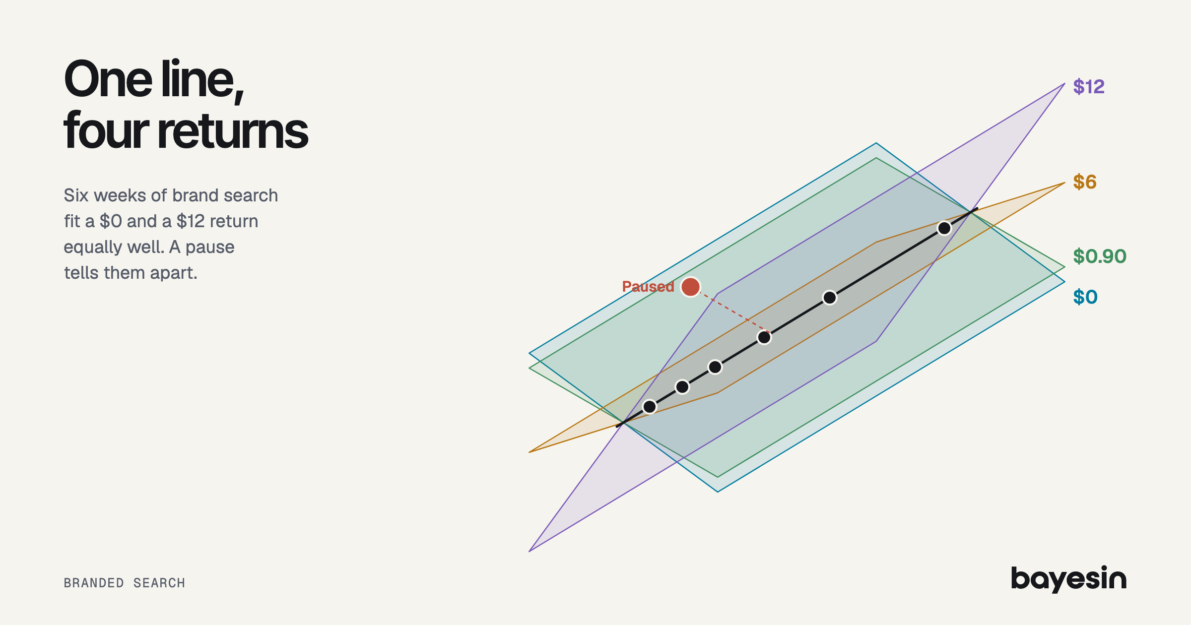
The same six weeks of data fit a $0 return on branded search and a $12 return, exactly. I built those weeks to show why this argument rarely ends. Platform ROAS looks high, someone in the room doubts it, and more history doesn't help.
The difficulty is that brand spend rises when demand rises, because the campaign buys the queries that arrive. So the data can't say which one moved revenue.
This post gives you a check to run on your own spend and a test design for your brand. It also reports a simulation of three fixes against a known answer. Every example here is synthetic, so none of it is customer data or a benchmark.
Is branded search incremental? Sometimes, and the size varies
Published results range from no measurable short-term benefit to clear lift, and the brand's position seems to explain part of that. No single figure carries over to your account.
The best-known result comes from eBay. In 2014, Blake, Nosko and Tadelis ran field experiments there. They found that "brand-keyword ads have no measurable short-term benefits," with natural search capturing 99.5% of the forgone click traffic when ads stopped. The authors only "suspect" this extends to other well-known brands, and it's a short-term read.
Organic position points the same way. In 2012, Google Research pooled 390 search ad pause studies. About 50% of ad clicks were incremental at organic rank 1, 82% at ranks 2 to 4, and 96% below that. Google sells these ads, the study is old and it counts clicks across all search. I'd use it for direction only.
Competition matters too, on vendor evidence. Haus, which sells testing, reports significant lift for 82% of high-competition brands and 35% of low-competition ones. Haus counts lift as significant when the probability it's above zero passes 80%. Stella's 2026 benchmarks, from 225 US direct-to-consumer geo tests, put the branded search median at 0.70x. Stella itself advises discounting those figures by 15-20% for planning.
Why can't a model settle it from spend and revenue?
Because spend moves with demand, many different returns fit equally well. Here are six synthetic weeks where spend is exactly $0.50 per query, since the campaign buys whatever arrives.
- 1: Brand queries: 20,000; Brand spend: $10,000; Revenue: $180,000
- 2: Brand queries: 24,000; Brand spend: $12,000; Revenue: $204,000
- 3: Brand queries: 22,000; Brand spend: $11,000; Revenue: $192,000
- 4: Brand queries: 31,000; Brand spend: $15,500; Revenue: $246,000
- 5: Brand queries: 38,000; Brand spend: $19,000; Revenue: $288,000
- 6: Brand queries: 27,000; Brand spend: $13,500; Revenue: $222,000
Now four stories, each of which reproduces all six revenue figures to the dollar.
- A: all demand: Revenue formula: $60,000 + $6.00 × queries; Return on spend: $0.00; If you stop the ads: Nothing changes
- B: all ads: Revenue formula: $60,000 + $12.00 × spend; Return on spend: $12.00; If you stop the ads: Most revenue goes
- C: half and half: Revenue formula: $60,000 + $3.00 × queries + $6.00 × spend; Return on spend: $6.00; If you stop the ads: A strong channel leaves
- D: mostly demand: Revenue formula: $60,000 + $5.55 × queries + $0.90 × spend; Return on spend: $0.90; If you stop the ads: Little is lost
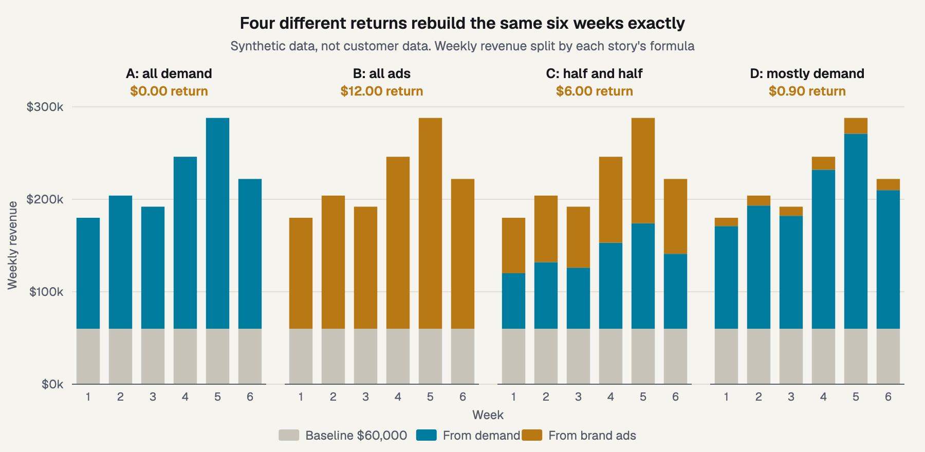
Figure 1. Every story rebuilds the same six weeks of revenue.
Queries and spend correlate at exactly 1.0 here. So any pair works where the query coefficient plus half the spend coefficient equals $6.00. More weeks like these wouldn't help, because the problem is the data's shape and not its size.
A real account has a correlation below 1.0 and a milder form of the same problem. In their 2017 Google paper, Chan and Perry draw two response surfaces that both fit such data well. They say selection bias "perhaps represents the largest hurdle" for these models, and they call paid search "a severe form" of it.
This differs from a channel whose spend never moves. Brand spend moves plenty, but it moves for the wrong reason.
Does a query-volume control fix it?
It removes much of the bias for search, and it can cost you accuracy elsewhere. A query control gives the model a separate measure of demand, so spend no longer has to stand in for it.
In a 2018 Google paper, Chen and colleagues report an "approximately unbiased estimate of search ad ROAS" in some common scenarios, compared with randomized experiments. Google's Meridian documentation says omitting query volume can lead to overestimating paid search. It also says "It is best to include these campaigns as separate media channels", so brand and generic each get their own line. Check the current page before you rely on that wording.
The cost sits in other channels. Meridian's control variables page says query volume is a confounder for search, and "a mediator" for other media that drive people to search. Mediators shouldn't be controls, and one model has to pick. So if video sends people to search your name, the control that helps brand search also hides part of video's effect.
Here's the check to run. Plot weekly brand spend against brand query volume, and look for weeks that leave the line, such as budget caps or freezes. Those weeks hold what the model can learn about the ads alone. If you find almost none, a control can't do much, and the next section shows why.
What happens when each fix is added?
Spend alone missed badly, a clean query control landed close, and a test prior was steadiest. Noise in the query series hurt more than I expected.
I simulated 500 synthetic brands over 104 weeks with a true return of 0.90. Demand follows a seasonal cycle, a persistent random drift and two shocks. Spend is $0.50 per query, capped at $18,000 a week, so the cap bound in 14.9% of weeks. A second run adds six random budget-freeze weeks at half spend.
The three models share seasonal terms and a weak prior on return, centered on 2 with a standard deviation of 4. The first uses spend and revenue only. The second adds the query control, at three noise levels. The third also takes a prior from a synthetic four-week pause in regions holding 30% of revenue, with a standard error of 0.49.
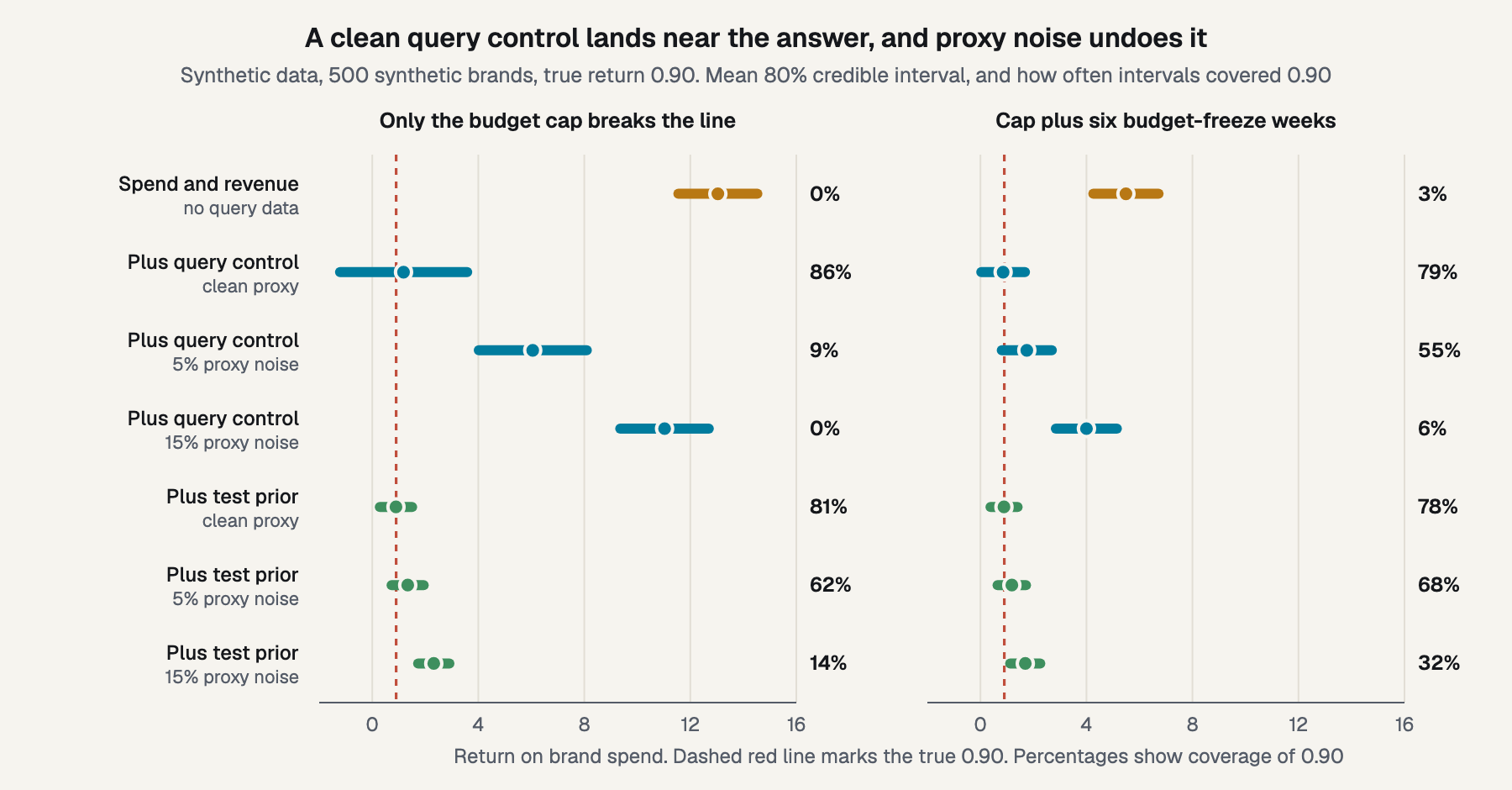
Figure 2. Three fixes against a known answer, with how often the 80% intervals covered 0.90.
Spend and revenue alone. The model averaged 13.04 with an interval from 11.55 to 14.53, and it covered 0.90 in 0% of brands. That's confident and wrong. Six freeze weeks cut it to 5.49, which still covered only 3% of the time.
The query control. With a perfect query series, it read 1.18 and covered 86% of the time, but the interval ran from -1.21 to 3.58. That width reflects how little the cap weeks teach. Centering the prior on 0.5 instead of 2 moved the read to 0.82, so the prior is doing visible work.
Noise changed the picture. With 5% noise in the query series, the read jumped to 6.06 and coverage fell to 9%. At 15%, it was 11.03 and 0%. I expected this to worsen with noise, but not this fast.
The reason is that spend tracks true queries almost exactly. A noisy proxy is then a worse record of demand than spend itself, so the model gives demand's credit to spend. The freeze weeks soften this: 1.75 at 5% noise and 4.00 at 15%.
The test prior. With a clean control it read 0.90 and covered 81% of the time, with an interval 1.22 wide. The test alone would give 1.26, so most of that precision came from the test. At 5% noise it read 1.34, and at 15% it read 2.32 with 14% coverage. A confident, biased fit can overrule a good test, so check the query series before you combine them. How a test result becomes a prior covers the mechanics.
Published work points the same way, with limits. In Google's 2024 simulations, Zhang and colleagues found that return priors from experiments can reduce bias and uncertainty. PyMC-Marketing's notebook warns that improvement "is not guaranteed" in every parameter. My own run is simpler than a real account: a constant return, no carryover or saturation, and weeks treated as independent. I look at what one test changes across a plan separately.
A credible interval states where the return lies given the model and its assumptions, so a wrong model can produce a narrow one. Coverage is a frequency across these 500 brands, and it isn't a property of any one interval.
I also turned on a video channel with a true return of 1.50, about half of it running through brand queries.
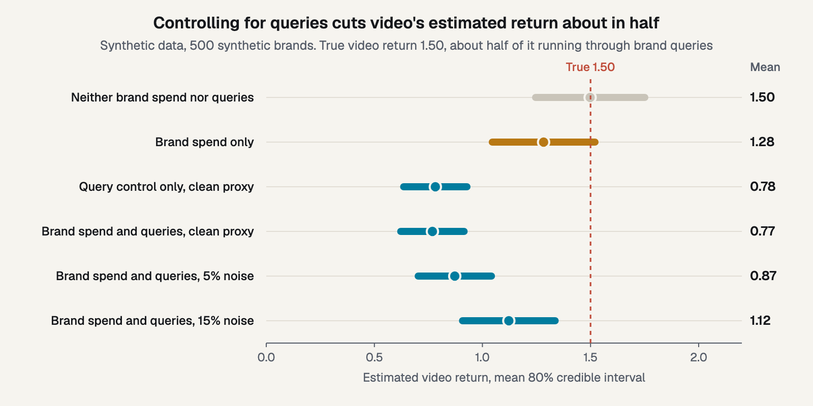
Figure 3. A query control removes the part of video's return that runs through search.
With a clean query control, video read 0.77 and its intervals never covered 1.50. Leaving out both brand spend and queries read 1.50 on average, though the intervals covered it only 59% of the time. That clean midpoint is partly by design, since video's flights ignore demand in this run. Keeping query volume and dropping the brand channel, a variant Chan and Perry show, still read 0.78.
How do you run a pause test that settles it?
Stop brand ads in randomly chosen regions and read total revenue, not paid clicks. A pause test is a lift test where the ads stop in some regions. It works because the pause moves spend without moving demand.
Say week 7 has 28,000 queries across two regions of 14,000, with a regional baseline of $30,000. One region spends $7,000 and the other pauses. The running region earns $114,000 under every story, while the paused region separates them.
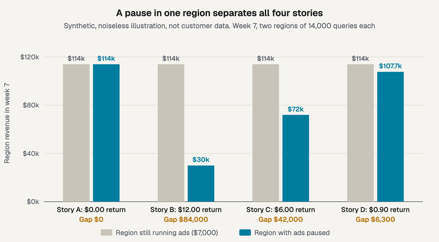
Figure 4. One paused region gives four different answers.
Under story D, the gap of $6,300 on $7,000 of spend returns the $0.90. This is a noiseless illustration of why a pause identifies the return. Two regions and one week can't support a real read. In 2015, Lewis and Rao found a median confidence interval on ad return over 100 percentage points wide across 25 display ad experiments. Story D's paused region falls just 5.5%, and that's the size of effect a real test must detect.
So plan it with care:
- Pick the regions at random. See choosing and matching regions.
- Size it. Work out how big a test needs to be.
- Plan a window after the pause. Decide how long to run the pause before you start. Haus reports a median brand test of 14 days, and only 27% had a post-treatment window.
- Record the context first. Note competitor presence and your organic rank, since both can shape the result.
- Read every sales channel. A click lost in paid search may reappear in organic, direct or stores.
My simulated four-week pause has a detectable return of 1.38, using the 2.8 multiplier (two-sided 5%, 80% power). That's above the true 0.90, and it has 45% power against zero. Against a break-even of 1.82, though, 72% of its 80% intervals fall fully below the line. Often the question is about break-even, and zero is only one reference point.
What a holdout measures that credit can't covers the wider argument, and marketing incrementality testing covers the whole method. Your team runs the test, since Bayesin never changes spend.
What do you do with the result?
Compare the return with 1 over margin, then decide. At a 55% margin, break-even return at your margin is 1 / 0.55 = 1.82, and story D's 0.90 misses it.
Here's that arithmetic at 28,000 queries a week. Spend is $14,000 and incremental revenue is $12,600, so lost margin at 55% is $6,930. Pausing keeps $7,070 a week before any reallocation. A 7.5 platform ROAS would report $105,000 on that spend, so the incremental share is 12%.
Three outcomes follow:
- The interval sits below break-even. Cut or reduce the bids, and watch competitors.
- The interval sits above break-even. Keep it, and stop relitigating it each quarter.
- The interval crosses break-even. Treat it like an interval that crosses zero: a range to plan with, and possibly a bigger test.
Retest when a competitor starts bidding on your name or your organic rank changes. Then feed the result to the model as a prior, after you've checked the query series.
Frequently asked questions
Should I stop bidding on my brand?
Only after a test, because the answer depends on your competitors and organic rank. The eBay result came from one very well-known brand. Your result can also change later, for example when a rival starts bidding on your name. So treat a pause as a decision you may revisit.
Why is branded ROAS so high?
It counts people already on their way to you. Someone searching your name was likely to buy anyway, and the platform still credits the click. In the synthetic example, a 7.5 platform ROAS sits on top of a 0.90 return, so only 12% of reported revenue is incremental.
Should branded search be in my model?
Usually yes, separated from generic search and with a query control, provided the query series is clean. Note the trade-off for video and other upstream channels, because one model has to choose. If your spend never leaves the query line, the model needs a test to learn much.
How long should a pause run?
Long enough for the delayed effect to finish, plus a window after the ads return. Haus reports a median of 14 days for brand tests, which leaves little room for that. Set the length and the read date before you start, and hold to them.
What to do next
Plot your brand spend against your query volume this week, and count the weeks that leave the line. Then ask whether your query series is clean enough to trust. If either answer is weak, plan a pause.
Bayesin shows what the next dollar returns in each channel, as marginal return with an 80% credible interval. Where the model knows least, it designs the test. Your team runs it, and Bayesin tracks it and reads the result. If you'd like to see that on your own channels, you can request access.
Sources
- NBER, "Consumer Heterogeneity and Paid Search Effectiveness: A Large Scale Field Experiment," Blake, Nosko and Tadelis, working paper, 2014
- UC Berkeley Haas, "Consumer Heterogeneity and Paid Search Effectiveness: A Large Scale Field Experiment," authors' copy, 2014
- Google Research, "Impact of Organic Ranking on Ad Click Incrementality," blog post, 2012
- Google, "Challenges And Opportunities In Media Mix Modeling," Chan and Perry, 2017
- Google, "Bias Correction For Paid Search In Media Mix Modeling," Chen et al., 2018
- Google for Developers, "Paid search modeling," Meridian documentation, 2026
- Google for Developers, "Control variables," Meridian documentation, 2026
- Google Research, "Media Mix Model Calibration With Bayesian Priors," Zhang et al., 2024
- PyMC-Marketing, "Lift Test Calibration," documentation
- Quarterly Journal of Economics, "The Unfavorable Economics of Measuring the Returns to Advertising," Lewis and Rao, 2015
- Haus, "When Is Branded Search Worth the Investment?," vendor research, 2025
- Stella, "2025 DTC Digital Advertising Incrementality Benchmarks," vendor benchmarks, 2026
See it on your own rows.
Bayesin is pre-launch. Join the waitlist and we will reach out as access opens.
Get new posts by email.
New posts only. See privacy for what we keep.