B2B
Media mix modeling for B2B: pipeline, lag and closed-won
Media mix modeling for B2B, worked through: a closed-won specification with lag set from your own deal cycle, plus checks for few deals and long waits.
Brandon Cade · Nov 2, 2026 · 20 min read
Key Takeaways
- Media mix modeling can work for B2B, and four checks from a CRM export show how far.
- One synthetic closed-won fit, at 78 deals a year, left ranges wide.
- Carryover cut LinkedIn's spend variation from 66% to 9%.
- Priors move the baseline share, so state them, and test where the dollars are large.
A co-founder of Recast, a measurement vendor, titled a 2026 article Why Media Mix Modeling So Rarely Works for B2B. His reasons are solid: few deals, long waits and validation that can take years. So I won't argue with the headline. I'd rather work the problem through with numbers you can check.
This post builds one closed-won specification, setting by setting. It gives you four numbers to compute from your own CRM and spend exports. Then it fits the specification to a seller where I know the truth. You'll see what the fit gets right and what it can't learn.
The seller is synthetic and so is every result here, so none of this is customer data. The specification is a teaching example, not a description of how Bayesin is built.
Does media mix modeling work for B2B?
It can, in the sense that it narrows some ranges and tells you how wide the rest are. Four checks from your own data show how much narrowing to expect, and how much will come from your priors instead.
The case against is strong, and it's from a competitor, so treat it as directional. Michael Kaminsky describes an enterprise firm closing ten deals a quarter, on cycles of 12 to 24 months. One contract can be 40% of a quarter's revenue. With 18-month cycles, he notes, holdout validation could take years. He places the workable cases at roughly $1,000 to $10,000 in contract value, with shorter cycles.
Rampmetrics, another vendor, makes the same point: "The longer and lumpier the cycle, the harder it is". It says B2B cycles often run 3 to 18 months.
The method still has one lasting advantage. It uses aggregate spend and revenue, with no user tracking, which matters in a long buying process with many people. I compare the two in attribution and media mix modeling.
So treat "does it work?" as four numbers rather than a yes or no about your category.
- Deal count: How to compute it: Weekly CV / sqrt(weeks); This seller: 9.8% at 156 weeks; If it falls short: Model converted pipeline, or lean on tests
- Lag against history: How to compute it: Spend weeks before the first outcome week, against your 90th percentile; This seller: 26 against 25.2; If it falls short: Backfill spend, or accept thin early weeks
- Spend variation: How to compute it: CV of raw and carried-over spend; This seller: LinkedIn 66% raw, 9.1% carried; If it falls short: Add variation on purpose
- Outcome stability: How to compute it: Did "won" or close date change meaning?; This seller: Stable by construction; If it falls short: Break the series, or add a control
None of these has a universal pass mark. The one fixed number I'd use is the flat-spend check, which flags a coefficient of variation below 15%. That check looks at raw spend, and applying it to carried-over spend is my own extension.
This seller looks fine on the first two checks and falls below that line on the third for every channel, as the next sections show. If you're still deciding whether to start at all, read whether a model is worth it yet.
What does a worked closed-won specification look like?
Here's every setting on one page, with where it came from and when to change it. I haven't found a vendor page that gives a closed-won specification with values, though one may exist.
The seller. It sells mid-market software through reps and closes 1.5 deals a week, or 78 a year. Deal size is lognormal with a median of $36,000 and a sigma of 0.9, so the mean is $53,975. That makes weekly revenue about $80,962, or $4.21 million a year. It has no deal at all in 22.3% of weeks.
The spend. Five channels share $26,000 a week: LinkedIn Ads $9,000, paid search $7,000, webinar sponsorships $4,000, review sites $3,000 and display retargeting $3,000.
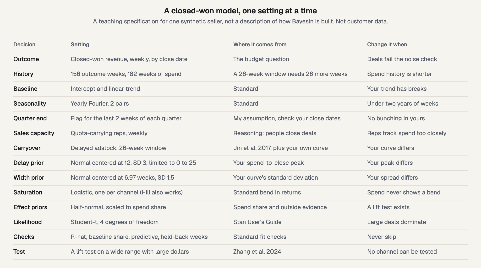
Figure 1. The specification card. This is a teaching specification, not a description of how Bayesin is built.
How to read the card. The outcome is closed-won revenue by close date, weekly. The baseline is an intercept and a trend, plus yearly seasonality, as I cover in baseline and seasonality. Two settings are specific to selling through people. A quarter-end flag covers the last two weeks of each quarter, and a weekly count of quota-carrying reps covers sales capacity. Both are my assumptions, so check them against your own close dates.
Carryover is delayed adstock over 26 weeks, and saturation is logistic, one curve per channel. If those terms are new, start with adstock and saturation. Effect priors are half-normal and scaled to spend share, and how priors work explains why. The likelihood is Student-t with four degrees of freedom, which Stan's guide describes for regression that tolerates outliers.
The count. The card has 12 independent variables: five channels, a trend, four Fourier terms, the quarter-end flag and reps. Robyn's analyst guide suggests a ratio of one variable to ten observations, which asks for 120 weeks. This history of 156 weeks gives 13 weeks per variable, so the rule is met.
Parameters tell a harder story. Each channel carries an effect, a delay, a width and a saturation, which makes 20. Add eight for the baseline and one for noise, and you have 29, or 5.4 weeks each. That's why the priors matter so much, and the 2017 Google paper by Jin and colleagues makes the same point about small samples. Sharing delay and width across channels cuts the count to 21, or 7.4 weeks each. I expected that to help, and the fit below says otherwise.
Which outcome goes in the model?
Closed-won answers the budget question, and pipeline gives the earlier read. Report on closed-won where your deal count can carry it, and keep pipeline as a working signal that comes first.
Keep your quantities apart before you pick. Konabayev's B2B guide puts it plainly: "Separate created pipeline, won contracts, recognized revenue and received cash." Those four move on different clocks. A weekly file that mixes them will blur the lag you're trying to measure.
Pipeline works as a stand-in only under a condition. Athey, Chetty, Imbens and Kang set out the surrogate condition, in a job-training setting, so this is an analogy. The treatment's effect on the long-term outcome has to pass through the stand-in. If one channel brings opportunities that close far less often than another's, pipeline will flatter it.
For the same reason, one blended win rate can misprice channels. It assumes every channel's opportunities convert alike, which is the thing you'd want to check first. Convert pipeline by channel if your CRM lets you.
Tools handle this in different ways. Meridian's data class takes a revenue_per_kpi value by geo and time, so you can model a count and price it. Robyn's guide says the dependent variable varies by vertical. Both leave the choice to you.
How far back does spend reach?
As far as your own spend-to-close curve reaches, which is further than common defaults. So build the curve first, then set the window from it.
Building the curve. On this seller, first touch to opportunity is lognormal with a median of 3 weeks and a sigma of 0.8. Opportunity to won is lognormal with a median of 11 weeks and a sigma of 0.45. I assume spend and first touch land in the same week. Added together, the median is 15.0 weeks, the 80th percentile 21.1 and the 90th percentile 25.2. The weekly histogram peaks at week 12.
Only 5.9% of closes land within 8 weeks, and 36.3% within 13.
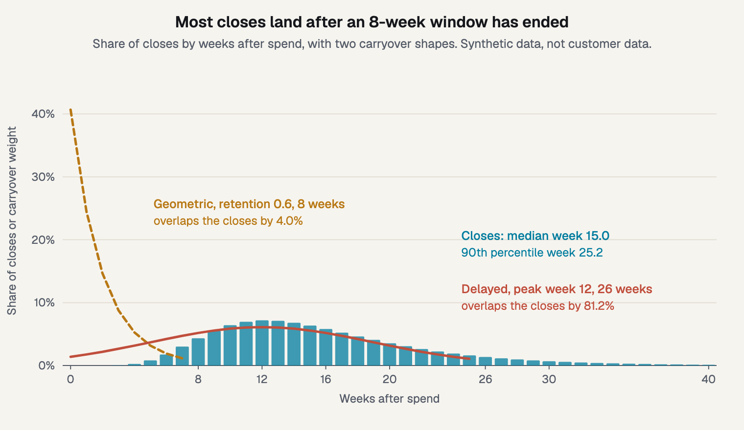
Figure 2. The closes against two carryover shapes.
The shape matters as much as the length. Count overlap as the smaller value in each week. A geometric curve with a retention of 0.6 over 8 weeks then shares just 4.0% with this histogram. A delayed curve with a peak at week 12 and a 26-week window shares 81.2%. Jin and colleagues explain why: geometric decay peaks at exposure, while a delayed form can peak later. Their own example used 13 weeks, for shampoo.
Open-source defaults are written for shorter cycles. Meridian's guidance recommends a max_lag of 2 to 10 for geometric decay and 4 to 20 for binomial. It also truncates effects there and assumes decay is monotonic. Robyn's features page recommends Weibull PDF for longer conversion windows. These pages can change, so check the current versions before you rely on them.
Setting the window. I set the window at about the 90th percentile, as a working choice. Here that's 25.2 weeks, so I used 26, which leaves 8.7% of closes outside it. Use the curve's peak and standard deviation as the centers of your priors, here 12 and 6.97 weeks. Delay and width priors then carry your CRM's knowledge into the model.
Counting the deals properly. Don't build the curve from won deals alone, because recent spend hasn't had time to close. Open deals and lost deals both carry information. Therneau, Crowson and Atkinson's survival tutorial labels censoring the other endpoint "a bad idea", and it uses Aalen-Johansen estimates for competing outcomes. Their examples are clinical, but won and lost deals have the same structure.
The cost in history. A 26-week window needs 26 weeks of spend before your first outcome week. So this card uses 182 weeks of spend for 156 of outcomes. Meridian's reference notes that short media history gets imputed as zero, so check what your tool does.
The larger cost took me by surprise. A long, wide curve averages spend over months, which removes most of the variation a model learns from.
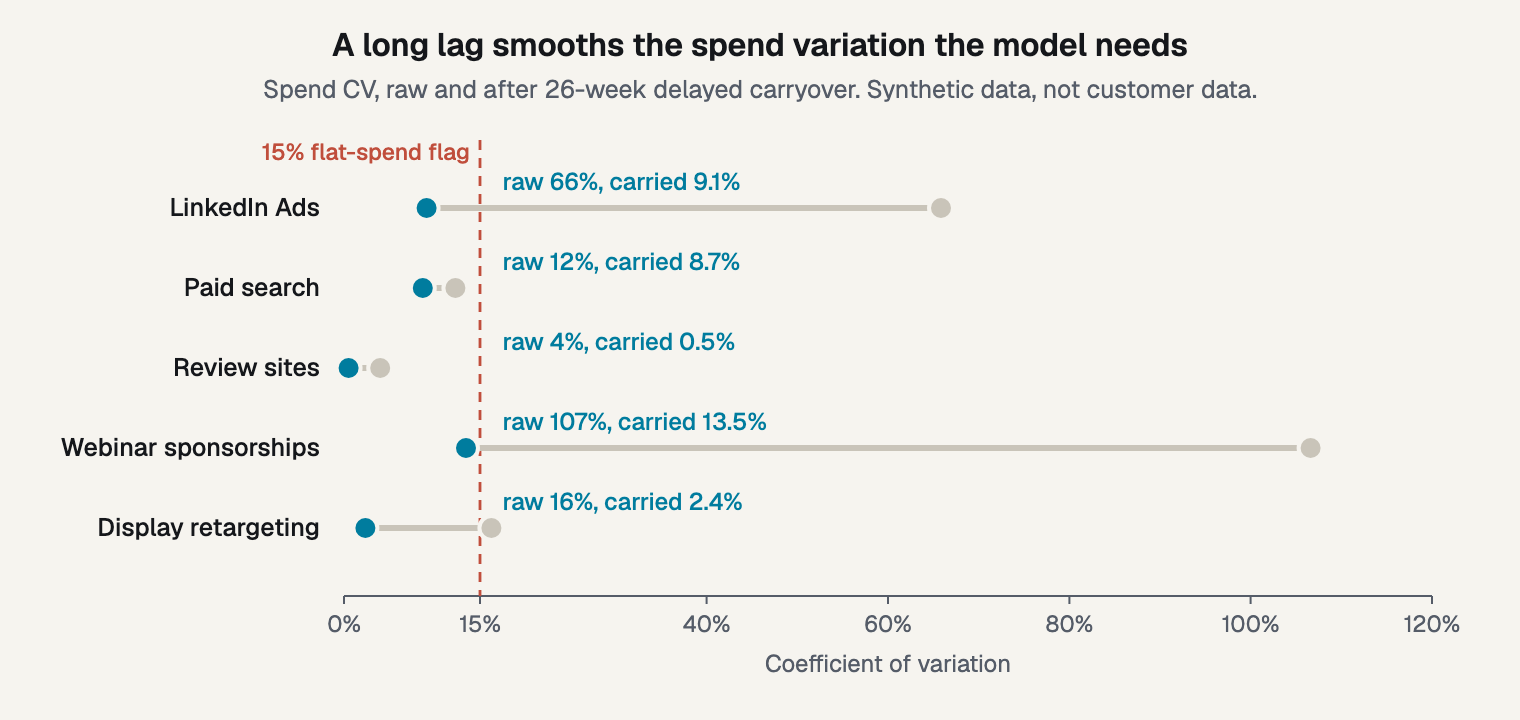
Figure 3. Bursts that look large on a weekly chart mostly disappear after carryover.
LinkedIn's bursts give it a coefficient of variation of 66% on a weekly chart, and carryover takes that to 9.1%. Webinars fall from 107% to 13.5%. All five channels end below the 15% line, and a raw check would have passed LinkedIn and webinars easily. Run this one on carried-over spend.
How do you model a few large deals?
Compute the noise floor first, then choose a likelihood that a single deal can't steer. The floor tells you how small a change in average revenue your history can show at all.
Noise floor is the weekly coefficient of variation divided by the square root of weeks. Weekly CV squared equals (1 + deal-size CV squared) / deals per week. Here deal-size CV squared is 1.248, so the weekly CV is 1.22.
At 78 deals a year, the noise floor is 17.0% at 52 weeks, 12.0% at 104 and 9.8% at 156. So three years of history still leaves about a tenth of average revenue as noise, before the model tries to split anything among five channels. These are calculated from the synthetic settings, and yours will follow your own deal count and spread.
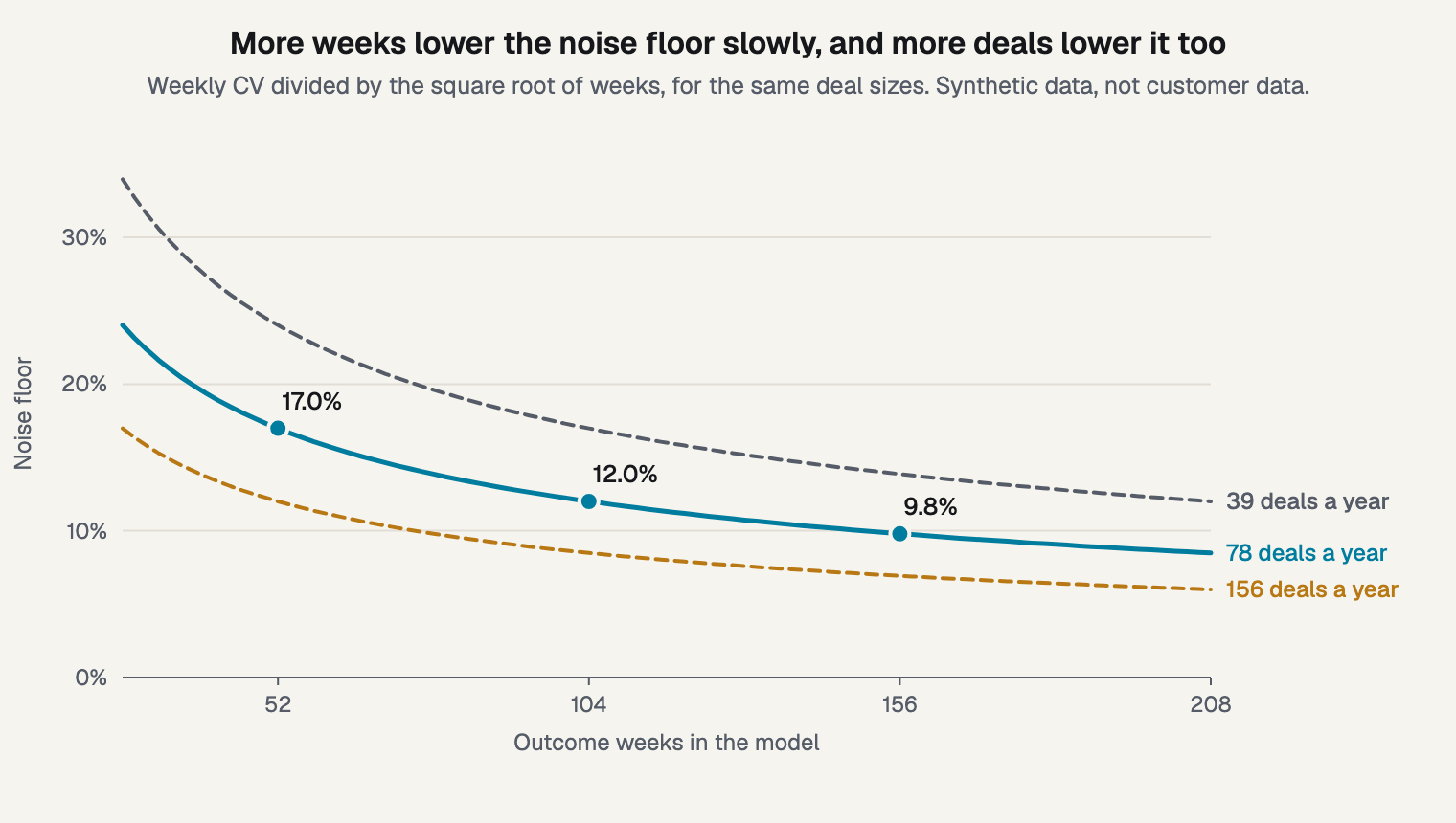
Figure 4. Doubling the deals lowers the floor as much as doubling the weeks.
Rolling up to months doesn't help. Monthly CV is lower, at 58.8%, but you have only 36 months, and 58.8% / sqrt(36) is the same 9.8%. You've smoothed the chart without adding any information. You also lose the weekly detail the lag needs.
For the likelihood, the card uses Student-t, so one large week doesn't pull the fit as hard as it would under a Normal. It has a cost, though. On revenue this skewed, Student-t centers below mean revenue, at about 80% of it in this fit. So returns read low: LinkedIn came to $0.79 here, against $0.98 under a Normal on the same draw. Measure baseline share against actual revenue, not that center, or it reads far too low.
If a few contracts dominate your revenue, a two-part model may suit you better. One part covers deal counts and the other covers deal sizes. That idea has a long history in insurance. Smyth and Jorgensen's 2002 paper uses Poisson arrivals with gamma costs, so treat it as an analogy.
Deals this size are ordinary even on a mid-market seller. The largest week in the synthetic draw holds 41% of an average quarter's revenue, close to Kaminsky's example. I ran Student-t and a Normal here, but not a two-part version, so I can't tell you what that would change. Look at your own largest weeks before you decide, and read how many weeks a model needs for the wider question.
What does a fit of this specification show?
It shows wide ranges that sit close to the priors. The fit doesn't rank the channels, and the baseline share still moves with the scale of the effect prior. That's useful to know before anyone reads a number off it.
I drew 182 weeks of spend, with bursts on LinkedIn and webinars. Deals arrive as Poisson counts, with rates from the baseline, quarter end, reps and each channel's saturated spend through the Figure 2 histogram. This draw has 256 deals over 156 weeks. I set the true baseline share at 58%. The true marginal returns came out at $1.03 for LinkedIn, $1.24 for search, $1.29 for review sites, $0.86 for webinars and $0.38 for display. Marginal return is the closed-won revenue from one more dollar a week at current spend.
The sampler behaved. The largest R-hat was 1.008 across the fits at normal noise, and 1.024 on one low-noise check. The card had no divergences. Those are checks on the sampler, and they don't say the answer is right. That's why six checks on a fit goes well beyond them.
At 78 deals a year, the delay came from the prior. The fit put the delay at week 12.3. Its 80% credible interval ran from 8.7 to 16.2. That looks like a recovery, until you change the prior. With a flat delay prior the interval ran from 3.4 to 23.0, close to the flat prior's own spread. With a prior centered on week 6, the delay stayed at 6.4.
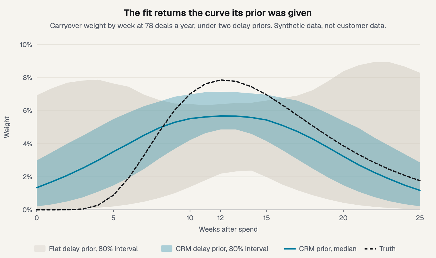
Figure 5. At 78 deals a year, the data alone can't place the curve, so your CRM has to.
So at this deal count, the spend-to-close curve can't be learned from the fit. The good news is that you can measure it directly from your CRM, as above.
Noise is the reason. I reran the same bursts with weekly noise cut to about 6% of mean revenue, which takes about 600 deals a week. A flat prior then placed the delay at 13.3, from 12.1 to 14.6. A prior on week 6 came back at 12.5, against a true 12. Long flights did worse at that noise, with a prior on week 6 ending at 7.7. So the data can place the delay only when bursts swing revenue well above the noise, and a seller with few deals doesn't get that.
Channel returns stayed near the priors. A credible interval is the range a value likely falls in, given the model and its priors. It says nothing about whether the model is right, as I cover in reading a credible interval. Here, the data narrowed LinkedIn's interval by 45% against the priors alone, and paid search's by 43%. The three small channels narrowed by only 21%, 25% and 21%.
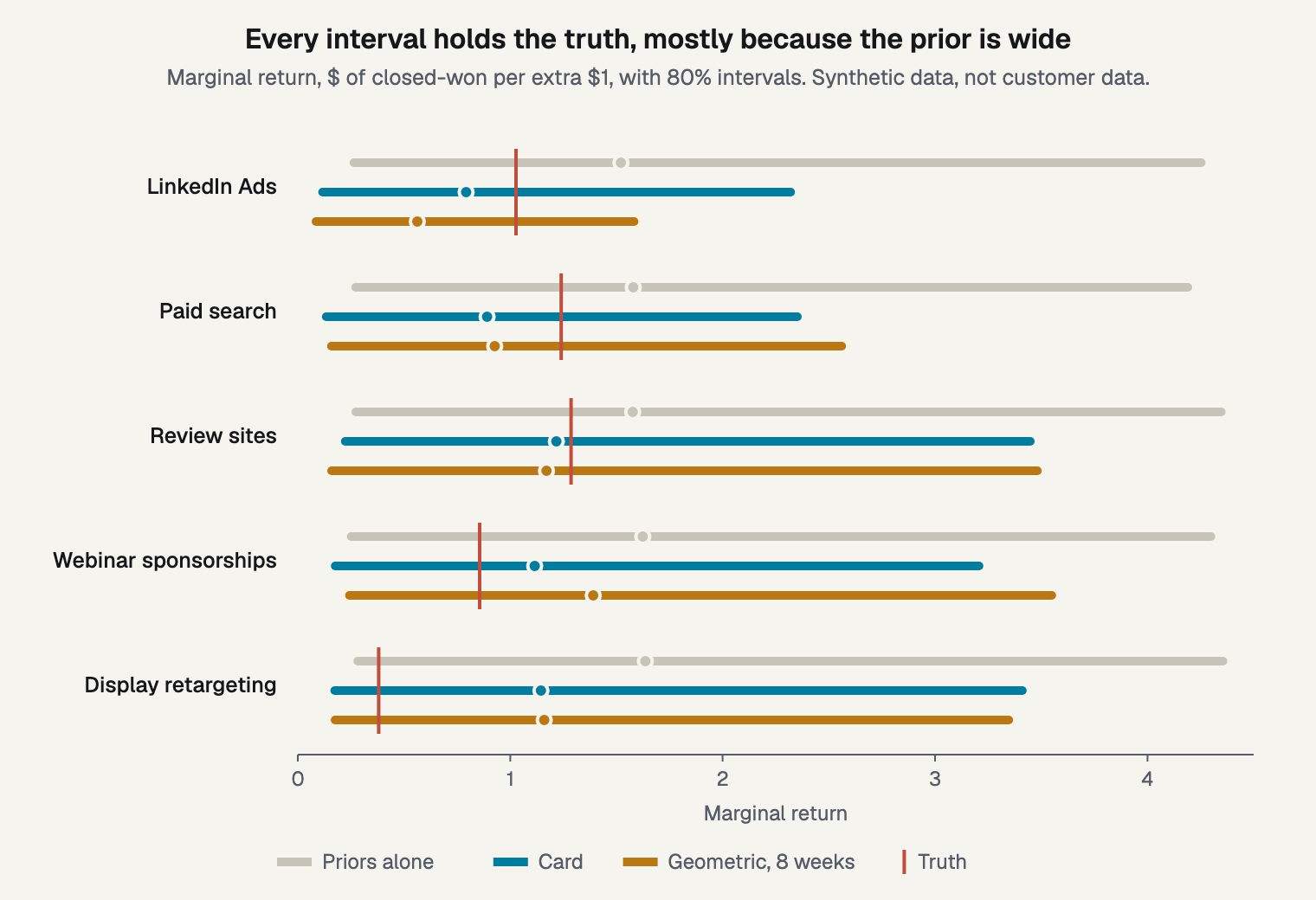
Figure 6. Every interval holds the truth, and few are narrow enough to rank channels.
Every interval contains the truth, yet the order is wrong. Display has the lowest true return at $0.38, and its median is $1.14, above LinkedIn's $0.79. I then repeated the fit on 10 more synthetic worlds, and all 50 of the 80% intervals held the truth.
That isn't good calibration. All 50 true values, from $0.37 to $1.29, also sit inside the priors' own 80% intervals, which run from about $0.27 to $4.30. A calibrated interval misses one time in five only on average across worlds drawn from its prior. These worlds all sit in the middle of it, so 50 of 50 says the ranges are wide, not that they're accurate.
The baseline share moved with the effect prior. The truth is 58%, and the fit says 51%, with an 80% interval of 26% to 72%. The data did real work here. Priors alone say 16%, from -46% to 55%, and 35% of those draws have media exceeding all revenue.
But the data didn't pin down the split. When I halved the scale of the effect prior, the fit moved to 65%. When I quartered it, the fit moved to 80%, with an interval of 65% to 89% that misses the truth. So treat the split as partly a choice you've made. I cover what to look for in six checks on a fit.
The 8-week geometric version. It raised the baseline share to 57% in this draw. Across the 10 extra worlds it was higher in all 10, averaging 56% against 51%. That sits nearer the truth by far less than either interval's width, and its timing is wrong, so I wouldn't count it as a win. LinkedIn's median fell to $0.56, as I'd expect for a bursty channel, but webinars rose to $1.39. Across the 10 worlds, LinkedIn fell in 5 and rose in 5, so I can't say geometric understates bursty channels in general.
Held-back weeks didn't separate the two versions either. On the last 13 weeks, the error was $144,256 against $146,904, and 9 of 13 weeks fell inside the 80% range for both.
What narrowed the ranges. I expected sharing delay, more deals and more spend variation each to help. The table shows the width of each 80% interval on marginal return, in dollars.
- Card, delay by channel: LinkedIn width: 2.20; Search width: 2.22; Baseline share: 51%
- Shared delay: LinkedIn width: 2.14; Search width: 2.35; Baseline share: 51%
- Ten times the deals, same revenue: LinkedIn width: 2.33; Search width: 2.47; Baseline share: 45%
- Long flights, carried CV about 40%: LinkedIn width: 2.04; Search width: 1.80; Baseline share: 55%
- Long flights and ten times the deals: LinkedIn width: 1.71; Search width: 1.72; Baseline share: 52%
Sharing delay changed almost nothing, because delay wasn't what held the ranges open. Ten times the deals, at a tenth of the size, narrowed only webinars, by 17%. Long flights, with 20 weeks high and 20 weeks low, narrowed three channels by 19% to 23%, and the other two by 4% and 5%. Both together narrowed LinkedIn, search and review sites by 20% to 28%, and left webinars and display about where they were.
The deals result has a plain reason: the data's own precision is still worse than the prior's. Ten times the deals cuts the noise floor from 9.8% to 3.1%. LinkedIn's carried spend varies by only 9.1%, so one standard error on its effect is about 34% of mean revenue. At $80,962 of weekly revenue and $9,000 of spend, that's about $3.06 per dollar. An 80% interval from that alone is nearly $8 wide on average return, against about $4 for the prior on marginal return.
It takes far more. At a hundred times the deals, LinkedIn's width fell from 2.14 to 0.74 and webinars' from 3.02 to 1.56, the two channels with bursts. Search and review sites didn't narrow, and display narrowed 15%. One seller and one set of priors can't settle this for everyone. If yours looks similar, plan to carry wide ranges and say so.
How do you test when you sell to accounts?
Assign accounts where you can target them and regions where you can't, and expect a range rather than a verdict on small lists. On this seller, a test's value depends far more on the dollars it moves than on how wide the interval is.
Tests matter more here than in ecommerce, for a simple reason. Kaminsky notes that forecast-based validation can take years on long cycles. A test gives you outside evidence without that wait. Zhang and colleagues at Google found in simulation that calibration can reduce bias and uncertainty in posterior return. For the full method, read marketing tests, from pick to use. I also study what one test changes in a Bayesian model.
Tests are hard, though. In 2015, Lewis and Rao found a median interval on return over 100 percentage points wide across 25 experiments, in retail and brokerage. A B2B seller has far fewer buyers than they did. Here's the arithmetic for this seller, with half its regions dark for 26 weeks and a closed-won read over 52.
The noise on the difference comes to $714,707. Display withholds $39,000, so its standard error on return is 18.3, while LinkedIn withholds $117,000, for a standard error of 6.1. Display has the widest interval, which makes it the obvious test candidate. I added that test to the fit through a term on average return. PyMC-Marketing's lift term reduces to that when a test takes spend to zero. Its interval barely moved.
A test with a standard error of 0.5 would change that. Display's interval narrowed by 80%, its median fell from $1.14 to $0.27, and the truth of $0.38 stayed inside. The baseline share also rose from 51% to 55%. But reaching 0.5 on a closed-won read would take about $1.43 million of withheld spend, on a channel that spends $3,000 a week.
An earlier outcome is the practical route. Suppose you read converted pipeline on LinkedIn over 26 weeks, at an assumed 25% win rate. The standard error falls to 2.16. I fit that twice, with the read landing as far below the truth as above it.
The low read of -$0.51 narrowed LinkedIn's interval by 31% and moved its median to $0.54. The high read of $2.91 narrowed it by 1% and moved its median to $1.00. Most of that 31% came from the zero bound in the prior, so don't plan on it. PyMC-Marketing warns that improvement "is not guaranteed", and that's what I saw here.
Where the model knows least, Bayesin designs the test. Your team runs it, and Bayesin tracks it and reads the result. It never changes your spend.
Frequently asked questions
Does MMM work with a long sales cycle?
It can, if you set the lag from your own cycle and your spend history covers it. On this seller, a delayed 26-week curve overlaps closes by 81.2%, and a geometric 8-week curve by 4.0%. At this deal count the fit can't find that curve alone, so measure it from your CRM.
How much data does a B2B MMM need?
Weeks and deals both count, and so does spend variation. At 78 deals a year, three years leaves a noise floor of 9.8%. Spend history has to run longer than outcomes, by the length of your window. Compute the floor from your own deal count and spread before you scope anything.
Can I use leads or pipeline instead of revenue?
Yes, if the channel's effect on revenue passes through that stand-in. That's the surrogate condition, and it fails when channels' opportunities close at different rates. Convert pipeline by channel where you can, and keep the win rates you used on the page. Then report closed-won later as a check.
Does a B2B MMM replace attribution?
No, because they answer different questions. On Bayesin for B2B, the model explains closed-won revenue, and attribution across funnel stages credits every stage before it. Attribution shows the path a deal took. The model estimates what spend caused, at the level of weeks, without tracking any one person.
What if my deals are too few?
Use three fallbacks. Model converted pipeline, run tests on your largest channels, and use account analytics for the enterprise deals, as Kaminsky suggests. You can still fit a model, but expect it to reflect your priors. Say so, show the ranges, and don't rank channels on medians.
Pull your four numbers
Start with one export from your CRM and one from your ad accounts. Compute your noise floor, your 90th percentile from spend to close, your carried-over spend variation and any change in what "won" means. Those four tell you what a model can teach you, and where your priors or tests have to do the work.
Bayesin models the revenue you closed, week by week, including the months between the spend and the signed deal. It works from weekly revenue, not deal counts, so with few deals its ranges will be wider, and it shows you how wide.
Sources
- Google Research, "Bayesian Methods for Media Mix Modeling with Carryover and Shape Effects," Jin et al., 2017
- Google Research, "Media Mix Model Calibration With Bayesian Priors," Zhang et al., 2024
- Google Meridian, "Set the max_lag parameter," documentation, 2026
- Google Meridian, "meridian.data.input_data.InputData," API reference, 2026
- Meta Robyn, "Key Features," documentation, 2026
- Meta Robyn, "An Analyst's Guide to MMM," documentation, 2026
- NBER, "The Surrogate Index," Athey, Chetty, Imbens and Kang, 2019, revised 2024
- R survivalVignettes, "Competing Risks and Multistate Models," Therneau, Crowson and Atkinson, 2024
- ASTIN Bulletin, "Fitting Tweedie's Compound Poisson Model to Insurance Claims Data: Dispersion Modelling," Smyth and Jorgensen, 2002
- PyMC-Marketing, "Lift Test Calibration," documentation, 2026
- Quarterly Journal of Economics, "The Unfavorable Economics of Measuring the Returns to Advertising," Lewis and Rao, 2015
- Stan User's Guide, "Regression Models," reference, current edition
- MarTech Series, "Why Media Mix Modeling So Rarely Works for B2B," by Michael Kaminsky of Recast, opinion, 2026
- Rampmetrics, "Is Marketing Mix Modeling For You?," vendor page, 2026
- Konabayev, "Marketing Mix Modeling (MMM) for B2B Companies," consultant's guide, 2026
See it on your own rows.
Bayesin is pre-launch. Join the waitlist and we will reach out as access opens.
Get new posts by email.
New posts only. See privacy for what we keep.